Reconstruct Tracks connects time-sequential points into tracks and summarizes records within the track. Tracks are identified by one or more track fields. The resulting DataFrame contains the track as a linestring or a polygon, the count of records within a track that have been summarized, and any additional statistics that have been specified.

Usage notes
-
Reconstruct Tracks requires point or polygon geometries. The input DataFrame must be time enabled with records that represent an instant in time.
-
You can specify one or more fields to identify tracks using
set. Tracks are represented by the unique combination of one or more track fields. For example, if theTrack Fields() flightandID Destinationfields are used as track identifiers, the recordsI,D007 SoldenandI,D007 Tokyowould be in different tracks since they have different values for theDestinationfield. -
Records that have a buffer applied will result in polygonal tracks. Input points that do not have a buffer applied will result in linestring tracks.
-
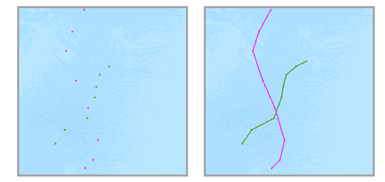
Input DataFrames must be time-enabled and represent an instant in time. Results are linestrings or polygons that represent an interval in time. The start and end of the interval are determined by the time at the first and last records in a track.
-
An input DataFrame with two distinct tracks (green and red) that have time type instant (left) and resulting tracks with time type interval (right) are shown.
-
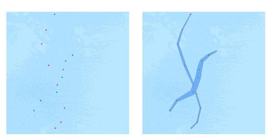
You can optionally apply a buffer to your input points. When you apply a buffer, the resulting tracks will be polygons.
-
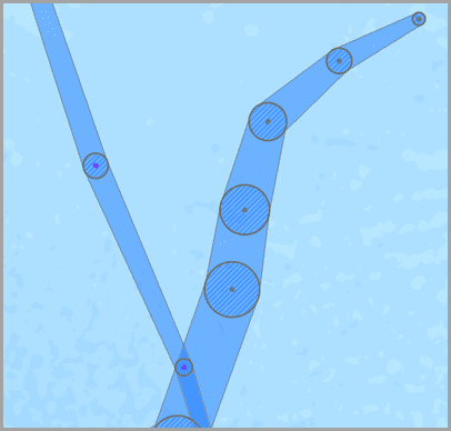
When buffering input points, each point is buffered. Then a convex hull is generated to create a polygonal track.
-
For linestring results, only tracks that contain more than one point will be returned. If you apply a buffer, all inputs will be returned.
-
Fields used in the buffer expression must be numeric and will be applied using the units of the input's spatial reference. See Arcade expressions for more information. You can use track-aware equations.
-
By default, only the count of points or polygons in a track will be calculated. Optionally, use
addto calculate additional numeric statistics (count, sum, minimum, maximum, range, mean, standard deviation, variance, first, and last) or string statistics (count, any, first, and last) for the rows summarized within a track.Summary Field() -
By default, tracks are created using the planar distance method when the input DataFrame is in a projected coordinate system and the geodesic distance method when the input DataFrame is in a geographic coordinate system. To override this default behavior, use
set. It is recommended that you use geodesic distance in the following circumstances:Distance Method() - Tracks crossing the international date line—When using the geodesic method, input DataFrames that cross the international date line will result in tracks that correctly cross the international date line. Your input DataFrame or processing spatial reference must be set to a spatial reference that supports wrapping around the international date line, for example, a global projection such as World Cylindrical Equal Area.
- Buffers—Input records can optionally be buffered.
-
You can split tracks in the following ways:
-
set- Splits tracks based on a time between input records. Applying a time split breaks up any track when input data is farther apart than the specified time. For example, if you have five records with the same track identifier and the times ofTime Split() [01and set a time split of 2 hours, any records that are measured more than 2 hours apart will be split. In this example, the result would be a track with:00, 02 :00, 03 :30, 06 :00, 06 :30] [01and:00, 02 :00, 03 :30] [06, because the difference between 03:30 and 6:00 is greater than 2 hours.:00, 06 :30] -
set- Splits tracks based on defined time intervals. Applying a time boundary split segments tracks at a defined interval. For example, if you set the time boundary to 1 day, starting at 9:00 a.m. on January 1, 1990, each track will be truncated at 9:00 a.m. every day. This split accelerates computing time, as it creates smaller tracks for analysis. If splitting by a recurring time boundary makes sense for your analysis, it is recommended for big data processing.Time Boundary Split() -
set- Splits tracks based on a distance between input records. Applying a distance split breaks up any track when input data is farther apart than the specified distance. For example, if you set a distance split of 5 kilometers, sequential records greater than 5 kilometers apart will be part of a different track.Distance Split() -
set- Splits tracks based on an Arcade expression. Applying a split expression splits tracks based on values, geometry or time values. For example, you can split tracks when a field value is more than double the previous value in a track. To do this, using an example field namedArcade Split() Wind, you can use the following expression:Speed var speed = Track. Tracks will split when the previous value (Field Window(' Wind Speed', -1, 1); 2\* speed[0] \ < speed[1] speed[0]) is less than two times the current value.
-
-
You can apply none, one, two, three, or four split options at the same time. All of the examples below use a gap split. The results, assuming you apply a time split of six hours, a time boundary of one day, and distance split of 16 kilometers, are as follows:
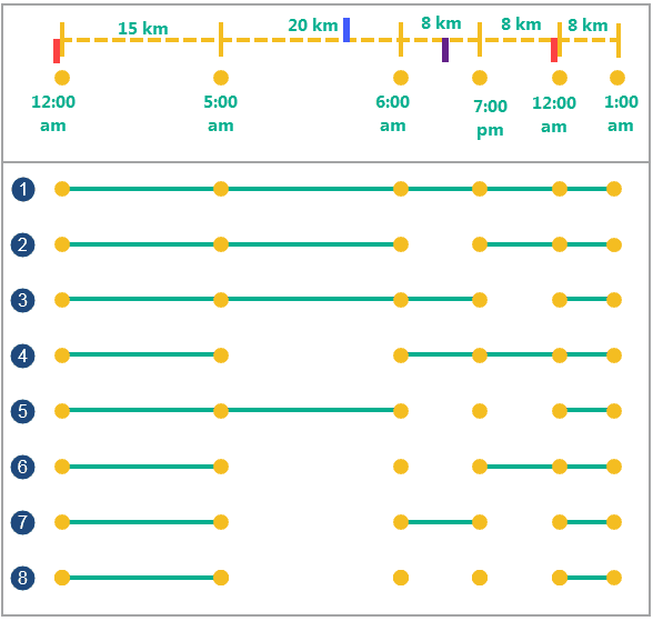
Split option Description Six input points with a time and location. Input points with the same identifier. The distance between the points is marked on the top of the dotted line, and the time of each point measurement is marked below the points. There are four splits on the timeline. The red splits represent the time boundary split of 1 day, starting at 12:00 AM. The blue split represents the distance split, when the distance between two points is greater than 16 km. The purple split represents the time split, when the temporal distance between two sequential points is greater than 6 hours. 1. Example with no time split and no distance split. 2. Example with a time split of two hours. Any records greater than two hours apart are split into separate tracks. 3. Example with a time boundary of 1 day, starting at midnight. At each 1-day interval starting from the specified time (here 12:00 AM), a new track is created. 4. Example with a distance split of 16 kilometers. Any records greater than 16 kilometers apart (the records at 05:00 AM and 06:00 AM) are split into separate tracks. 5. Example with a time split of 6 hours and a time boundary of 1 day starting at 12:00 AM. Any records greater than six hours apart or that intersect with the time duration split at 12:00 AM are split into separate tracks. 6. Example with a time split of 6 hours and a distance split of 16 km. Any records greater than six hours apart (the records at 06:00 AM and 7:00 PM) or farther than 16 km apart are split into separate tracks. 7. Example with a distance split of 16 km and a time boundary of one starting at 12:00 AM. Any records greater than 16 km apart or that intersect with the time duration split at 12:00 AM are split into separate tracks. 8. Example with a distance split of 16 km, a time split of 6 hours, and a time boundary of one day starting at 12:00 AM. Any records greater than 16 km apart, or farther apart than 6 hours, or that intersect with the time duration split at 12:00 AM are split into separate tracks. -
When you split a track using a time split, distance split, or split expression, you can decide how segments between the split will be created. You have the following options:
- Gap—Create a gap between the two records that were split.
- FinishAfter—Create a segment that ends after the split.
- StartBefore—Create a segment that ends and starts before the split.
-
The following diagram shows an example of the split types:
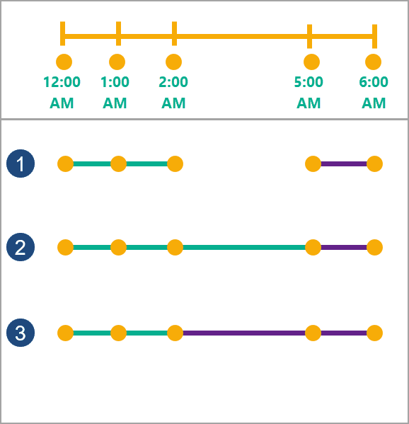
Three examples of time splits on the same input points (yellow) are shown.
Time split option Description Five input points with a time and location Five input points with the same identifier. The time of each point is marked below the dotted line. There is one split between 2:00 a.m. and 5:00 a.m. for all examples. Each track is split into two segments between the third and fourth points on the track. The first track is green and the second is purple. How the tracks are split is defined by setSplitType(). Gap (1) Example with a gap between the two points that are split. This is the default. Finish After (2) Example in which the track finishes after the split, at the fourth point. The second track starts at the fourth point. Start Before (3) Example in which the track splits before the split, at the third point. The second track starts at the third point. -
The following are examples of why it may make sense to define tracks using the split parameters and the field identifier parameter using an airline flight as an example: An aircraft record has
aircraft,ID flight,ID pilot,_name start, and_time flightfields. The_maneuver flightfield represents whether the aircraft is on land, ascending, descending, or at a constant altitude._maneuver -
Use the aircraft ID field as the identifier to see where each plane has traveled.
-
Use the aircraft ID and the flight ID fields as the identifiers to compare distinct routes.
-
Use the aircraft ID field and the time boundary of one year to examine the flights for each aircraft for a year at a time.
-
Use the pilot name, aircraft ID, and start time fields to view each pilot's flight.
-
Use the aircraft ID field as the identifier, and split distances farther than 1,000 kilometers, to determine new tracks, given that a 1,000-kilometer jump in measurements should not belong to the same track.
-
Use the aircraft ID field as the identifier and split using an expression when the value in the flight_maneuver field changes. For example,
var flight;_manuever = Track Field Window('maneuver', -1, 1) flightchecks whether the current value in a track and the previous value match. If not, the track is split._maneuver[0] != flight _maneuver[1]
-
Results
The tool outputs lines or polygons and includes the following fields:
| Field | Description |
|---|---|
TRACK | A field representing the duration of the track segment in milliseconds. |
track | The start time of the field. |
track | The end time of the field. |
<statistic | Specified statistics of specified fields. There are returned based on add inputs. |
COUNT | Count of records within a track. |
track | The output geometry that contains the track. |
Performance notes
Improve the performance of Reconstruct Tracks by doing one or more of the following:
-
Only analyze the records in your area of interest. You can pick the records of interest by using one of the following SQL functions:
- ST_Intersection—Clip to an area of interest represented by a polygon. This will modify your input records.
- ST_BboxIntersects—Select records that intersect an envelope.
- ST_EnvIntersects—Select records having an evelope that intersects the envelope of another geometry.
- ST_Intersects—Select records that intersect another dataset or area of intersect represented by a polygon.
- Don't apply a buffer.
- Split your tracks using one of the splitting options.
setwill have the biggest performance gains.Time Boundarysplit()
Similar functions
Syntax
For more details, go to the GeoAnalytics Engine API reference for reconstruct tracks.
| Setter | Description | Required |
|---|---|---|
add | Adds a summary statistic of a field in the input DataFrame to the result DataFrame. | No |
run(dataframe) | Runs the Reconstruct Tracks tool using the provided DataFrame. | Yes |
set | Sets an Arcade expression to split tracks with. The expression will be evaluated for each point in a track and the track will be split if the expression equals True. | No |
set | Sets a field in the input DataFrame that contains a buffer distance or a buffer expression. A buffer expression must begin with an equal sign (=). | No |
set | Sets the method used to calculate distances between track observations. There are two methods to choose from: ' or '. If this setter is not used, the geodesic distance method will be used when the input DataFrame is in a geographic coordinate system and the planar distance method will be used when the input DataFrame is in a projected coordinate system. | No |
set | Sets the distance used to split tracks. Any records in the input DataFrame that are in the same track and are farther apart than this distance will be split into a new track. If both the distance split and the time split are used, the track is split when at least one condition is met. | No |
set | Sets how the track segment between two points is created when a track is split. The split type is applied to split expressions, distance splits, and time splits. There are three options: ', ', and '. | No |
set | Sets boundaries to limit calculations to defined spans of time. | No |
set | Sets the time duration used to split tracks. | No |
set | Sets one or more fields used to identify distinct tracks. | Yes |
Examples
Run Reconstruct Tracks
# Log in
import geoanalytics
geoanalytics.auth(username="myusername", password="mypassword")
# Imports
from geoanalytics.tools import ReconstructTracks
from geoanalytics.sql import functions as ST
from pyspark.sql import functions as F
# Path to the Seattle example tracks data
data_path = r"https://services1.arcgis.com/36PP9fe9l4BSnArw/arcgis/rest/" \
"services/seattle_example_tracks/FeatureServer/0"
# Create a DataFrame from the Seattle example tracks data
df = spark.read.format("feature-service").load(data_path)
# Reconstruct tracks by user ID and return statistics for the horizontal accuracy column
result = ReconstructTracks() \
.setTrackFields("user_id") \
.setDistanceMethod(distance_method="Planar") \
.addSummaryField(summary_field="horizontal_accuracy", statistic="Min") \
.addSummaryField(summary_field="horizontal_accuracy", statistic="Max") \
.addSummaryField(summary_field="horizontal_accuracy", statistic="Mean",
alias="avg_horizontal_accuracy") \
.run(dataframe=df)
# Show a selection of columns and the length of the track for the first 5 results
result.select(ST.length(geometry="track_geometry").alias("length"), "user_id", "COUNT",
"TRACK_DURATION", F.round("avg_horizontal_accuracy", 13).alias("avg_horizontal_accuracy")) \
.sort("user_id", ascending=True).show(5)+------------------+-------+-----+--------------+-----------------------+
| length|user_id|COUNT|TRACK_DURATION|avg_horizontal_accuracy|
+------------------+-------+-----+--------------+-----------------------+
|32953.688189848006| user1|160.0| 160860000| 5.222359767449|
|18329.825427215314| user2| 82.0| 4860000| 4.8091253320749|
|30329.946152668355| user3|293.0| 106440000| 5.1580968157529|
| 39125.16386084201| user4|339.0| 96900000| 4.9619108295966|
|17847.608263107366| user5| 95.0| 5640000| 5.2804088837775|
+------------------+-------+-----+--------------+-----------------------+
only showing top 5 rowsPlot results
# Plot the Reconstruct Tracks result
result_plot = result.st.plot(cmap_values="user_id", is_categorical=True, cmap="Paired",
legend=True,
legend_kwds={"title": "User ID", "loc": "lower left", "bbox_to_anchor": (0, 0.03)},
figsize=(10,12),
basemap="light")
result_plot.set_title("Reconstructed user tracks")
result_plot.set_xlabel("X (US Survey Feet)")
result_plot.set_ylabel("Y (US Survey Feet)");Version table
| Release | Notes |
|---|---|
1.0.0 | Python tool introduced |