Extend GeoAnalytics with Custom Tools

The Run Python Script task executes a Python script on your ArcGIS GeoAnalytics Server site and exposes Spark, the compute platform that distributes analysis for GeoAnalytics Tools, via the pyspark package. A geoanalytics module is also available and allows you to run GeoAnalytics Tools within the script. You can use layers from ArcGIS Enterprise with both pyspark and geoanalytics as Spark DataFrames. To learn more, see Reading and Writing Layers in pyspark.

Below are several examples that demonstrate how you can integrate pyspark and geoanalytics to create powerful custom analysis.

Chaining GeoAnalytics Tools

By chaining together multiple GeoAnalytics tools in the Run Python Script task, you can automate analysis workflows and avoid creating unnecessary intermediate layers. In this example, multiple tools are used in succession and only the final result is saved.

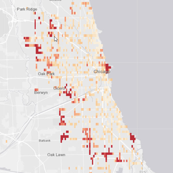
In this example, we will find hot spots of delayed buses. To do this, a big data file share dataset has been specified in the input_layers parameter of the Run Python Script task. It is available within the script at index 0 of the layers object. This dataset contains point locations of city busses recorded at 1 minute intervals for 15 days. Each point feature contains a status field called dly that is True if the bus is delayed and False in all other instances.

The Detect Incidents tool is first called within the script to identify, using an Arcade expression, all locations where a bus's delay status has changed from False to True. The result is returned in memory as a Spark DataFrame and used as input to the Find Hot Spots tool to identify hot spots of bus delay locations. The result of the Find Hot Spots tool is then written to the spatiotemporal big data store as a feature service layer.

Chaining together GeoAnalytics Tools to find hot spots of bus delay points.

Note: The purpose of the notebook is to show examples of the different tools that can be run on an example dataset.

from arcgis.geoanalytics.manage_data import run_python_script

def find_spots():
    import time
    
    # Create an Arcade expression to determine changes in value from False to True
    exp = "var dly = $track.field[\"dly\"].history(-2); return dly[0]==\"False\" && dly[1]==\"True\""

    # Run Detect Incidents to find all bus locations where delay status has changed from False to True
    delay_incidents = geoanalytics.detect_incidents(input_layer=layers[0], 
                                                    track_fields=["vid"], 
                                                    start_condition_expression=exp, 
                                                    output_mode="Incidents")

    # Use the resulting DataFrame as input to the Find Hot Spots task
    delay_hotspots = geoanalytics.find_hot_spots(point_layer=delay_incidents, 
                                                 bin_size=0.1, 
                                                 bin_size_unit="Miles", 
                                                 neighborhood_distance=1, 
                                                 neighborhood_distance_unit="Miles", 
                                                 time_step_interval=1, 
                                                 time_step_interval_unit="Days")

    # Write the Find Hot Spots result to the spatiotemporal big data store
    delay_hotspots.write.format("webgis").save("Bus_Delay_HS_{0}".format(time.time()))

run_python_script(find_spots, [input_layer]

After the script above has completed running, the result layer will be available in your Portal for ArcGIS contents. You can open the layer in a map and symbolize it on its z-score to visualize the resulting hot spots, as shown in the screen capture below.

Performing analysis with pyspark.ml

The pyspark package includes tools for distributed data management, regression, classification, clustering, and more. Many of these tools use DataFrames, allowing you to analyze ArcGIS Enterprise layers with pyspark functionality.

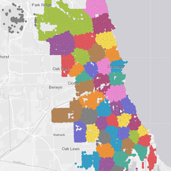
In the example below, the k-means algorithm is used to segment a map of crime data into a predefined number of clusters. You can then use this map to help efficiently dispatch officers throughout a city. The k-means algorithm is not included in GeoAnalytics Tools; however, it is included in the pyspark.ml package. By calling this implementation of k-means in the Run Python Script tool, you can execute k-means on your GeoAnalytics Server site using an ArcGIS Enterprise layer as input. You can then save the result as a feature service or other ArcGIS Enterprise layer type.

Using k-means to cluster crime events with the pyspark.ml package.

def clusters():
    from pyspark.ml.feature import VectorAssembler
    from pyspark.ml.clustering import KMeans

    # Crime data is stored in a feature service and accessed as a DataFrame via the layers object
    crime_locations = layers[0]

    # Combine the x and y columns in the DataFrame into a single column called "features"
    assembler = VectorAssembler(inputCols=["X_Coordinate", "Y_Coordinate"], outputCol="features")
    crime_locations = assembler.transform(crime_locations)

    # Fit a k-means model with 50 clusters using the "features" column of the crime locations
    kmeans = KMeans(k=50)
    model = kmeans.fit(crime_locations.select("features"))

    # Add the cluster labels from the k-means model to the original DataFrame
    crime_locations_clusters = model.transform(crime_locations)

    # Write the result DataFrame to the relational data store
    crime_locations_clusters.write.format("webgis").option("dataStore","relational").save("Crime_Clusters_KMeans")

run_python_scripy(clusters, [crime_lyr])

After the script above completes, the result layer is available in the Portal for ArcGIS contents. By symbolizing on the predictions made by the k-means model, you can visualize the clustered crime events as shown in the screen capture below.

This sample notebook can be referred for the above usecase.

Managing data with pyspark.sql

The pyspark.sql package supports running SQL queries and calculating statistics on DataFrames. This allows you to summarize, edit, and filter datasets in the Run Python Script tool before writing them out to a data store.

In the example below, a Living Atlas layer containing congressional district boundaries is converted to a DataFrame using its URL. pyspark is then used to calculate statistics on two columns in the dataset. These statistics are then used to query the dataset to find districts of interest before writing out the result to a big data file share.

Querying a layer using pyspark.sql.

def manage_data():
    # Specify the URL to the input layer
    districts_url = "https://services.arcgis.com/P3ePLMYs2RVChkJx/arcgis/rest/services/Congressional_District_Demographics/FeatureServer/0"

    # Load the feature service layer into a DataFrame
    districts = spark.read.format("webgis").load(districts_url)

    # Calculate the 90th percentile of household income, stored in a column called "MEDHINC_CY"
    income_percentile = districts.approxQuantile("MEDHINC_CY",[0.90],0.01)[0]

    # Calculate the average per capita income growth rate, stored in a column called "PCIGRWCYFY"
    income_growth_avg = districts.agg({"PCIGRWCYFY": "avg"}).collect()[0]["avg(PCIGRWCYFY)"]

    # Query for districts with a median household income in the top 10% and an income growth rate greater than average
    query_str = "MEDHINC_CY > {0} AND PCIGRWCYFY > {1}".format(income_percentile, income_growth_avg)
    districts_filtered = districts.filter(query_str)

    # Make a selection on the DataFrame to only include columns of interest
    districts_filtered_select = districts_filtered.select(["NAME","MEDHINC_CY","PCIGRWCYFY","$geometry"])

    # Write the result to ArcGIS Enterprise
    districts_filtered_select.write.format("webgis").option("dataStore","/bigDataFileShares/output_data:csv").save("Target_Districts")

run_python_script(manage_data)

After the script above completes, the result layer is available in your Portal for ArcGIS contents. By drawing the layer in a map, you can quickly identify the congressional districts that meet the criteria used to filter the original input layer.

Chaining GeoAnalytics and pyspark tools

As the GeoanAlytics and pyspark packages both work with Spark DataFrames, you can combine tools from each into a single analysis workflow.

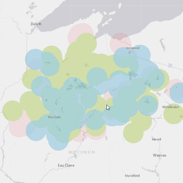
In the example below, a Naive Bayes classifier included with pyspark is trained to predict plant species using leaf and petal measurements. The classifier is applied to a dataset of unlabeled plant sightings to predict the species of each specimen. Afterward, the Create Buffers GeoAnalytics tool is used to create a map of habitat area for each plant species. The tool result is then written to ArcGIS Enterprise.

Chaining pyspark and geoanalytics tools to create a plant habitat map.

def classifier():
    from pyspark.ml.feature import StringIndexer
    from pyspark.ml.feature import VectorAssembler
    from pyspark.ml.classification import NaiveBayes
    from pyspark.ml import Pipeline

    # The input data is a table of labeled plant specimen measurements stored in a big data file share
    labeled_samples = layers[0]

    # Create a pipeline to prepare the data and train a Naive Bayes classifier with the labeled measurements table
    labelIndexer = StringIndexer(inputCol="Species", outputCol="label")
    vecAssembler = VectorAssembler(inputCols=["SepalLength", "SepalWidth", "PetalLength", "PetalWidth"], outputCol="features")
    nb = NaiveBayes(smoothing=1.0, modelType="multinomial")
    pipeline = Pipeline(stages=[labelIndexer, vecAssembler, nb])

    # Train the Naive Bayes classifier using the pipeline
    nb_model = pipeline.fit(labeled_samples)

    # Load a layer of unlabeled plant sightings with specimen measurements stored in a feature service
    unknown_samples = layers[1]

    # Predict plant species for the unlabeled sightings dataset using specimen measurements
    predictions = nb_model.transform(unknown_samples)

    # Create buffers around the plant sightings using the Create Buffers GeoAnalytics tool
    # By dissolving on plant species we obtain a map of approximate habitat area for each species
    species_areas = geoanalytics.create_buffers(predictions, distance = 10, distance_unit = "Feet", dissolve_option = "List", dissolve_fields = ["prediction"])

    # Write the result to the spatiotemporal big data store
    species_areas.write.format("webgis").save("plant_species_habitat_areas")

run_python_script(classifier, data)

After the script above completes, the result layer will be available in your Portal for ArcGIS contents. The layer contains a single polygon feature for each plant species identified by the Naive Bayes classifier, as shown below.

Writing results external to ArcGIS Enterprise

In many cases, it may be useful to write files directly to a local directory or shared folder. Files written in this way are not available in ArcGIS Enterprise. You can write to any location that the ArcGIS Server account has write access to.

In the example below, Random Forest regression is used to create a model of revenue using demographic information. Forest-based Classification and Regression is available in the geoanalytics package as well, but using the pyspark implementation, you can save the model that you create for use at a later time. A business can use this model to predict potential revenue in new customer areas. In this case, the root mean squared error of the model is printed out, a summary of feature importance is written to a text file, and the model is saved to a shared folder.

Persisting a model of customer revenue by saving to a shared folder.

def revenue():
    import os
    from pyspark.ml.regression import RandomForestRegressor
    from pyspark.ml.evaluation import RegressionEvaluator
    from pyspark.ml.feature import VectorAssembler

    # The training dataset is a feature service with the revenue and demographics of current customer areas.
    customer_areas = layers[0]

    # Combine explanatory columns into a single column called "features"
    assembler = VectorAssembler(inputCols=['mean_age', 'mean_fam_size', 'med_income', 'percent_edu'], outputCol='features')
    customer_areas = assembler.transform(customer_areas)

    # Split the dataset to keep 10% for model validation
    (trainingData, testData) = customer_areas.randomSplit([0.9, 0.1])

    # Create the Random Forest model and fit it using the training data
    rf = RandomForestRegressor(featuresCol="features", labelCol="pres_wmo_", numTrees=100, seed=14389)
    model = rf.fit(trainingData)

    # Apply the model to the test data removed earlier for validation
    predictions = model.transform(testData)

    # Calculate and print the Root Mean Squared Error between model results and actual revenue
    evaluator = RegressionEvaluator(labelCol="label", predictionCol="prediction", metricName="rmse")
    rmse = evaluator.evaluate(predictions)
    print("Root Mean Squared Error (RMSE) on test data = %g" % rmse)

    # Write a summary of feature importance to a shared folder
    out_path = r"\\data\rf\revenue_prediction"
    with open(os.path.join(out_path, 'feature_importance.txt'), 'w') as w:
        w.write(str(model.featureImportances))

    # Save the model to a shared folder for reuse
    model.save(os.path.join(out_path, 'model'))

run_python_script(revenue, data)

Thie sample notebook can be referred to for more information on this use case above.