Introduction
CycleGAN is and image-to-image translation model, just like Pix2Pix. The main challenge faced in Pix2Pix model is that the data required for training should be paired i.e the images of source and target domain should be of same location, and number of images of both the domains should also be same.
The Cycle Generative Adversarial Network, or CycleGAN, is an approach to training a deep convolutional neural network for image-to-image translation tasks. The Network learns mapping between input and output images using unpaired dataset. For Example: Generating RGB imagery from SAR, multispectral imagery from RGB, map routes from satellite imagery, etc.
This model is an extension of Pix2Pix architecture which involves simultaneous training of two generator models and two discriminator models. In addition to features of Pix2Pix, we can use unpaired dataset and also we can convert images in the reverse direction (target to source imagery) using the same model.
Model architecture

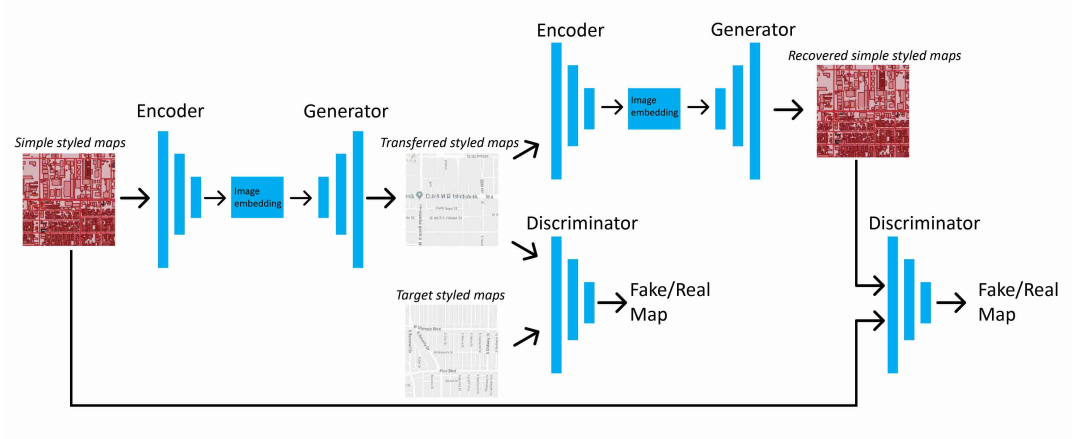
Figure 1. Overview of CycleGAN architecture: Translating from satellite image to map routes domain [3]
To know about basics of GAN, you can refer to the Pix2Pix guide.
The model architecture is comprised of two generator models: one generator (Generator-A) for generating images for the first domain (Domain-A) and the second generator (Generator-B) for generating images for the second domain (Domain-B).
- Domain-B -> Generator-A -> Domain-A
- Domain-A -> Generator-B -> Domain-B
Each generator has a corresponding discriminator model (Discriminator-A and Discriminator-B). The discriminator model takes real images from Domain and generated images from Generator to predict whether they are real or fake.
- Domain-A -> Discriminator-A -> [Real/Fake]
- Domain-B -> Generator-A -> Discriminator-A -> [Real/Fake]
- Domain-B -> Discriminator-B -> [Real/Fake]
- Domain-A -> Generator-B -> Discriminator-B -> [Real/Fake]
In arcgis.learn, all the discriminators and generators have been grouped into a single model.
How the loss is calculated while training?
The loss used to train the Generators consists of three parts:
- Adversarial Loss: We apply Adversarial Loss to both the Generators, where the Generator tries to generate the images of it's domain, while its corresponding discriminator distinguishes between the translated samples and real samples. Generator aims to minimize this loss against its corresponding Discriminator that tries to maximize it.
- Cycle Consistency Loss: It captures the intuition that if we translate the image from one domain to the other and back again we should arrive at where we started. Hence, it calculates the L1 loss between the original image and the final generated image, which should look same as original image. It is calculated in two directions:
- Forward Cycle Consistency: Domain-B -> Generator-A -> Domain-A -> Generator-B -> Domain-B
- Backward Cycle Consistency: Domain-A -> Generator-B -> Domain-B -> Generator-A -> Domain-A
- Identity Loss: It encourages the generator to preserve the color composition between input and output. This is done by providing the generator an image of its target domain as an input and calculating the L1 loss between input and the generated images.
*   Domain-A -> **Generator-A** -> Domain-A
*   Domain-B -> **Generator-B** -> Domain-B
As all of these loss functions play critical roles in arriving at high-quality results. Hence, both the generator models are optimized via combination of all of these loss functions.
Implementation in arcgis.learn
First, we have to export the image chips using Export Tiles format in arcgis pro, then create a databunch using prepare_data function in arcgis.learn
data = arcgis.learn.prepare_data(path=r"path/to/exported/data", dataset_type='CycleGAN')
The important parameters to be passed are:
- The
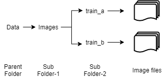
pathto the Data directory. We need to follow the directory structure shown in figure 2. Here, 'train_a' and 'train_b' folders contain the images of domain A and B.

Figure 2. Directory structure
- The
dataset_typeas 'CycleGAN'.
After creating the databunch, we can initialize CycleGAN object by calling
cyclegan_model = arcgis.learn.CycleGAN(data)
Unlike some other models, we train CycleGAN from scratch, with a learning rate of 0.0002 for some initial epochs and then linearly decay the rate to zero over the next epochs.
We can then continue with basic arcgis.learn workflow. For more information about the API & model, please go to the API reference.
References
[1] Jun-Yan Zhu, Taesung Park, Phillip Isola, Alexei A. Efros, “Unpaired Image-to-Image Translation using Cycle-Consistent Adversarial Networks”, 2017;arXiv:1703.10593.
[2] Jason Brownlee: Cyclegan Tutorial. Accessed 29 September 2020.
[3]. Kang, Yuhao, Song Gao, and Robert E. Roth. "Transferring multiscale map styles using generative adversarial networks." International Journal of Cartography 5, no. 2-3 (2019): 115-141.