Estimate stream runoff during a predicted rainstorm in Vermont.
Introduction
Stowe, a small Vermont town of nearly 5,000 residents, suffered considerably when the remnants of Hurricane Irene stuck the Green Mountain region in August 2011. The Little River overflowed and washed out roads, bridges, and culverts. Wanting to learn from the tragedy, Stowe officials discovered that they had precious little information involving flood prediction. They turned to hydrographs, which are line graphs determining how much water a stream will discharge during a rainstorm. In this notebook, you'll create those hydrographs.
Overwiew of the steps to be followed:

steps:
-
Remove imperfections in elevation model: Fill sinks in your elevation model to remove small imperfections in the data.
-
Delineate the watershed: Find the contributing area above a set of cells in an elevation model.
-
Create a velocity field: Determine how fast water flows with a spatially variant, time- and discharge-invariant velocity field.
-
Create an isochrone map: Assess the time it takes water to follow the flow path.
-
Create a unit hydrograph: Use the isochrone map to create a unit hydrograph for the outlet.
Necessary imports
from arcgis.gis import GIS
from datetime import datetime as dt

from arcgis.raster.functions.gbl import flow_direction, sink, fill, flow_accumulation, snap_pour_point, watershed
from arcgis.raster.functions import slope, raster_calculator, con
from arcgis.raster.analytics import convert_feature_to_raster
Connect to your GIS
gis = GIS('https://pythonapi.playground.esri.com/portal', 'arcgis_python', 'amazing_arcgis_123')Get data for analysis
The data is available here to download and can be published for completing the workflow.
We need the following layers layers include the following:
Pour_point—A point feature layer that depicts the outlet downstream of the Little River where you'll create a unit hydrograph.
Stowe_boundary—A polygon feature layer that depicts the boundaries of Stowe, Vermont. This layer was derived from data available from Vermont Center for Geographic Information (VCGI).
Stowe_surface_water—A raster layer that depicts all surface water bodies in the area of interest. This raster layer's resolution is 30 meters, which means that each cell in the layer has an area of 30 square meters. The layer was derived from features in the NHDPlus Version 2 dataset.
Stowe_DEM—A raster layer that depicts elevation within the study area. It also has a resolution of 30 meters. It was derived from data made available by the United States Geological Survey (USGS).
Stowe_velocity_example—A raster layer that depicts a spatially-variant, time- and discharge-invariant velocity field for the study area. You'll learn how to create this layer in a later lesson (this example is provided as a backup). For now, you don't need this layer, so it's turned off.
item = gis.content.get('36cbda7cabdb4933a60ee437f49da25b')itempour_point = item.layers[0]
stowe_boundary = item.layers[0]stowe_dem_item = gis.content.get('e8528b08a18b48958e16cc239d074e0d')
stowe_dem_itemstowe_dem = stowe_dem_item.layers[0]stowe_surface_water_item = gis.content.get('0abe2fe5b4694f08990907ce4ddcca62')stowe_surface_water_itemstowe_surface_water = stowe_surface_water_item.layers[0]m1 = gis.map('Stowe, Vermont')
m1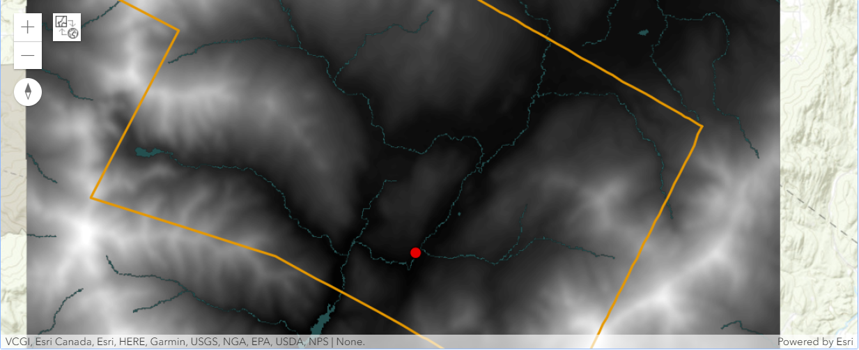
m1.add_layer(stowe_dem)m1.add_layer(stowe_surface_water)m1.add_layer(stowe_boundary)m1.zoom_to_layer(stowe_boundary)m1.add_layer(pour_point)Remove imperfections in elevation model
Some DEMs contain sinks, which are areas of low elevation surrounded by higher elevation values. Sinks can occur naturally but are more often data errors in a DEM raster dataset. Because water has no way of flowing out of a sink, sinks can cause all kinds of errors when analyzing how water flows to an outlet. Before you begin your hydrological analysis of flooding potential in Stowe, you'll identify and remove sinks from your elevation data.
Identify sinks
First, you'll identify sinks in your DEM. Although your DEM was derived from reliable data provided by the USGS, sinks may still be present. To run an accurate hydrological analysis for the area around Stowe, you'll first need to locate sinks if any.
stowe_flow_direction = flow_direction(stowe_dem).save('stowe_flow_direction' + str(dt.now().microsecond))stowe_flow_directionm2 = gis.map('Stowe, Vermont')
m2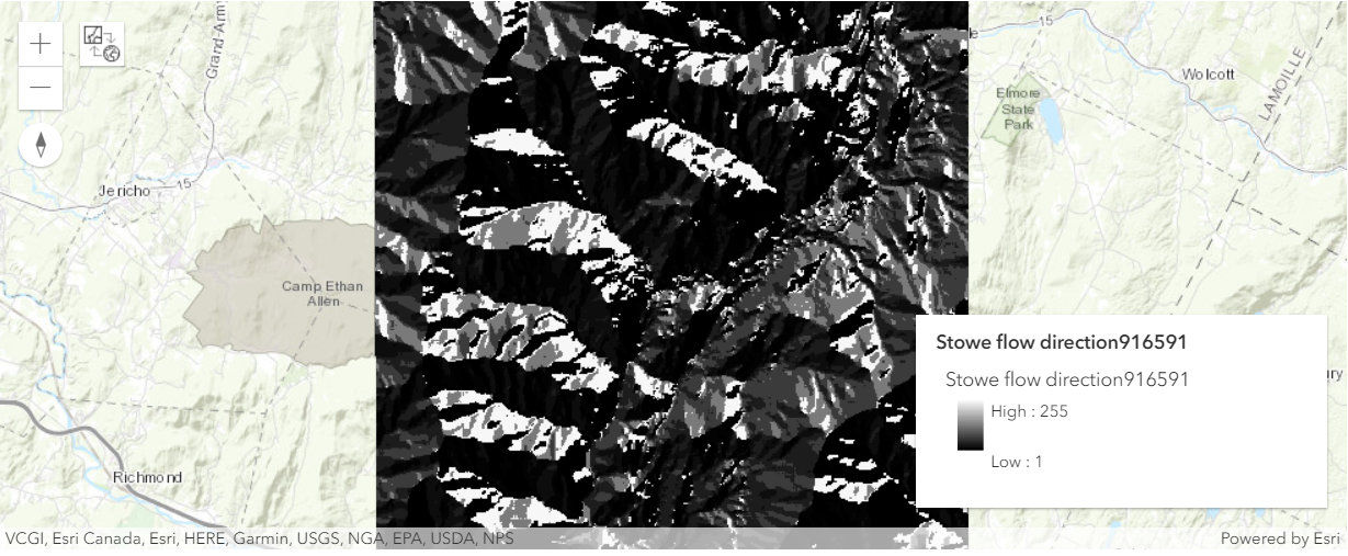
The symbology of the layer corresponds to the direction water is likely to flow, with darker colors indicating a more southerly flow direction and lighter colors indicating a more northerly flow direction. The layer's appearance isn't important to your analysis, because you'll run another tool that will automatically find sinks based on the flow direction layer.
m2.add_layer(stowe_flow_direction)
m2.zoom_to_layer(stowe_flow_direction)
m2.legend = TrueThe sink tool is used to identify areas of internal drainage (sinks) within the flow direction layer.
stowe_sinks = sink(stowe_flow_direction.layers[0]).save('Stowe_sinks' + str(dt.now().microsecond))stowe_sinksm3 = gis.map('Stowe, Vermont')
m3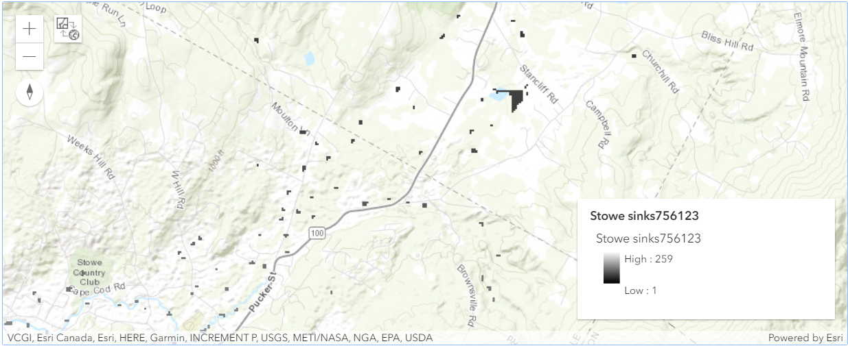
This map contains mostly small groups of black pixels, which might be difficult to see with its default symbology. You'll change the symbology to make the sinks easier to see.
m3.add_layer(stowe_sinks)
m3.zoom_to_layer(stowe_sinks)
m3.legend = Truefrom arcgis.raster.functions import colormap, stretchstowe_sinks_colormap = stretch(stowe_sinks.layers[0], dra=True)m4 = gis.map('Stowe, Vermont')
m4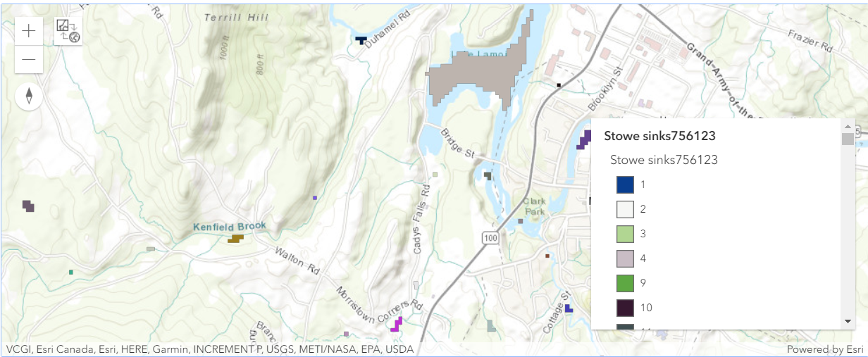
Sinks seem to appear primarily around stream networks and water bodies identified by the Stowe_surface_water layer. Existing water bodies tends to be flat and can cause errors in a DEM, such as sinks.
m4.add_layer(stowe_sinks_colormap)m4.zoom_to_layer(stowe_sinks_colormap)m4.legend = TrueFill sinks
Now that you've identified where sinks exist in your DEM, you'll create a DEM with the sinks removed using arcgis.raster.functions.gbl.fill(input_surface_raster, zlimit=None). In your new DEM, all sinks will be changed to have the elevation value of the lowest cell next to the sink. Each cell in the new DEM will be part of at least one continuous decreasing path of cells leading to an edge of the dataset. This new DEM will allow for more accurate hydrological analysis of the Stowe region.
stowe_fill = fill(stowe_dem).save('stowe_fill' + str(dt.now().microsecond))The final parameter, Z limit, allows you to set a maximum elevation difference (between a sink and its pour point) at which to fill sinks. If the difference in elevation between a sink and its edge is above the limit, the sink won't be filled. You want to fill all of the sinks in your data, so you'll leave this parameter unchanged.
m5 = gis.map('Stowe, Vermont')
m5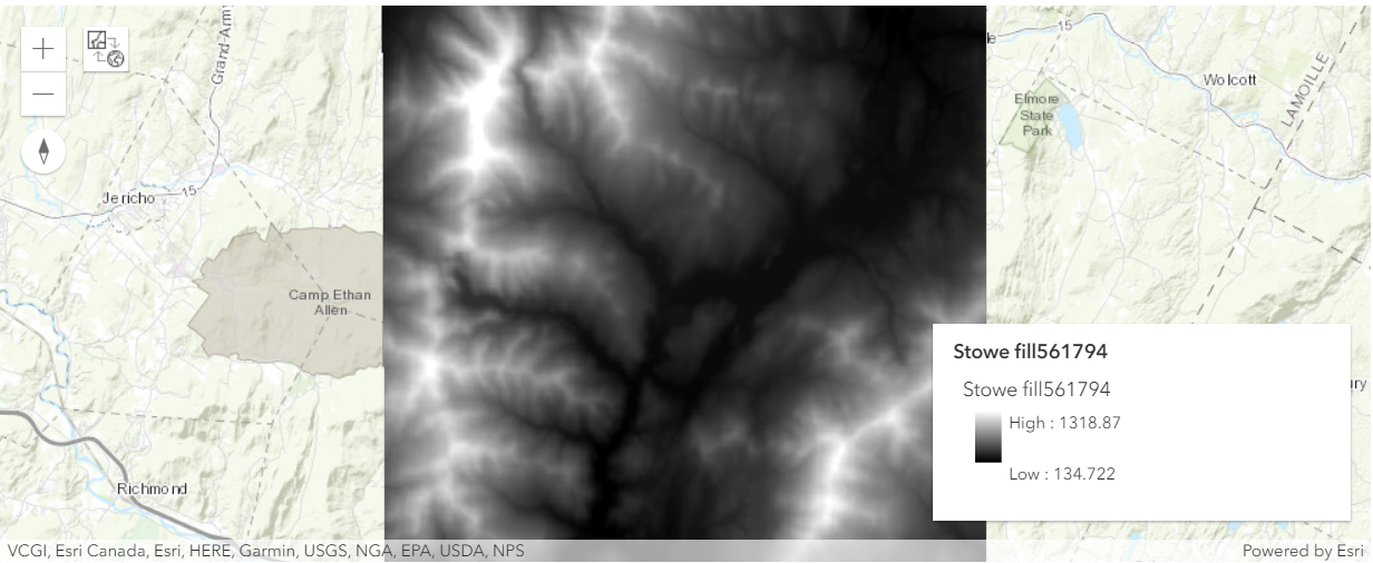
It looks almost identical to the original DEM, but the sinks in the dataset have been filled. You'll use this layer as the basis for your subsequent analysis of hydrological conditions in and around Stowe.
m5.add_layer(stowe_fill)
m5.zoom_to_layer(stowe_fill)
m5.legend = TrueYou've used a series of raster tools to identify sinks within a raw DEM. By inspecting the sinks, you might have also found that most of them occurred on or close to surface water bodies, likely due to insufficient elevation data. Lastly, you have filled the sinks in the dataset. Next, the newly created DEM is to be used to determine the watershed that spans Stowe, in order to help determine how water accumulates around the town.
Delineate the watershed
Previously, you removed sinks from your DEM to make it ready for hydrological analysis. Next, you'll use your DEM to determine the watershed area for the outlet point south of Stowe. A watershed area is the area in which all flowing water will flow toward a certain point—in this case, your outlet. With the watershed area, you'll be able to limit your subsequent analysis results to the relevant area for your outlet. Determining a watershed requires two components: a flow direction raster layer and an accurate outlet point.
Assess flow directions
The first step to delineate a watershed is to determine the direction that water will flow in your DEM. That way, you can determine the areas where water will flow to the outlet. To do so, you'll create another flow direction raster layer using flow_direction tool, this time for your DEM with filled sinks.
stowe_fill_flow_direction = flow_direction(stowe_fill.layers[0],
                                           flow_direction_type='D8',
                                           force_flow='NORMAL').save('Stowe_fill_flow_direction' +
                                                                      str(dt.now().microsecond))
m6 = gis.map('Stowe, Vermont')
m6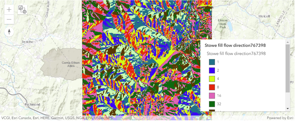
Unlike the previous flow direction layer, which was symbolized in black and white, this layer is symbolized with color (the specific colors used are random and may differ from the example images).
m6.add_layer(stowe_fill_flow_direction)
m6.zoom_to_layer(stowe_fill_flow_direction)
m6.legend = TrueThe cell values in a flow direction raster layer can normally be one of only eight integers: 1, 2, 4, 8, 16, 32, 64, and 128 as shown here. These eight integers correspond to the eight possible flow directions (as any given cell is surrounded by eight cells). Your previous flow direction layer, however, had some values that weren't one of those eight integers. Those values belonged to the sinks that you later removed from the data. Because the original flow direction layer had a wide range of values, it was automatically symbolized based on a color ramp, which uses the default black-to-white color scheme. Your new flow direction layer only has eight values, so it was automatically symbolized with a unique color for each value.
Snap outlet to stream
With your flow direction layer, you have the first component for determining a watershed. The other component is the location of an outlet point. One of the layers that you downloaded with the project is the pour_point layer, which represents an outlet downstream of Stowe, Vermont. For an accurate watershed, the outlet must be precisely located on the stream as rendered in the DEM (which may differ slightly from the actual location of the stream due to the DEM's resolution or other inaccuracies). First, you'll determine the stream's exact location by calculating the areas where water accumulates the most. Then, you'll snap the outlet point's location to match the stream exactly.
flow_accumulation tool creates a raster layer that indicates where water is most likely to accumulate. The flow_accumulation for each cell is expressed as a numeric value based on the number of cells that flow into that cell. Cells with high values of accumulation often coincide with the locations of flowing water bodies. With your flow accumulation raster, you'll identify the Little River that flows through Stowe.
stowe_flow_accumulation = flow_accumulation(stowe_fill_flow_direction.layers[0]).save('Stowe_flow_accumulation' +
                                                                                      str(dt.now().microsecond))
m7 = gis.map('Stowe, Vermont')
m7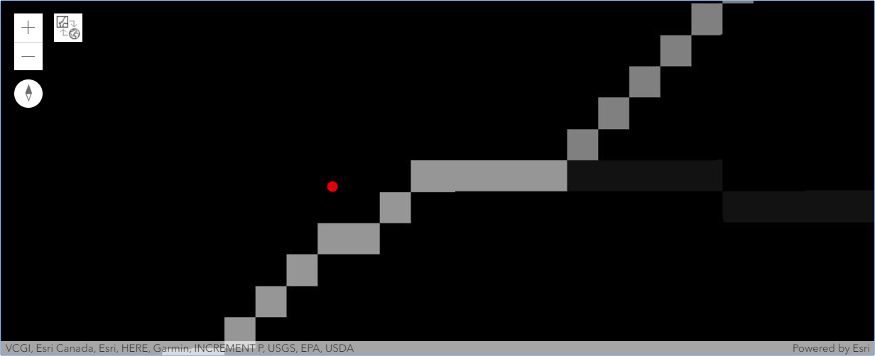
The cells with the highest flow accumulation are white. The faint line of white cells that runs through the outlet point is the Little River.
m7.add_layer(stowe_flow_accumulation)
m7.zoom_to_layer(stowe_flow_accumulation)m7.add_layer(pour_point)We want to Snap pour point to the cell of highest flow accumulation within a specified distance. The snap_pour_point tool requires an input raster layer to be snapped. Since, you have pour_point as a feature layer, you will conver it to rester using convert_feature_to_raster tool.
pour_point_raster = convert_feature_to_raster(pour_point,
                                              output_cell_size={"distance":30,"units":'meters'},
                                              value_field='objectid',
                                              output_name='pour_point_raster' + str(dt.now().microsecond))
You'll use measure tool available in ArcGIS Online Maps to measure the distance between the current outlet point and the Little River's location as represented in the flow accumulation raster. You can use this distance to then snap the outlet point to the correct cell so that it precisely lines up with the stream.
The measurement is approximately 50 meters (it may vary slightly, but an approximation is fine). Based on the measurement, you'll use a distance of 60 meters when you snap the outlet point to the stream. A snapping distance that is slightly higher than the measured distance will help avoid ambiguity in the tool. When deciding on a snapping distance, be sure it doesn't exceed the measured distance by too much, or the point may snap to an area further downstream.
stowe_snapped_outlet = snap_pour_point(pour_point_raster.layers[0],
                                       pour_point_field='value',
                                       in_accumulation_raster=stowe_flow_accumulation.layers[0],
                                       snap_distance=60).save('Stowe_snapped_output' + str(dt.now().microsecond))
m8 = gis.map('Stowe, Vermont')
m8
It looks like a pixel is missing in the flow_accumulation layer, however the output of the stowe_snapped_outlet is overlaid over the former raster.
m8.add_layer(stowe_flow_accumulation)
m8.zoom_to_layer(stowe_flow_accumulation)m8.add_layer(pour_point)m8.add_layer(stowe_snapped_outlet)Delineate watershed upstream of outlet
Now that you have both a flow direction layer and an accurate outlet layer, you can determine the watershed area upstream of the outlet.
stowe_watershed = watershed(stowe_fill_flow_direction.layers[0],
                            stowe_snapped_outlet.layers[0]).save('StoweWatershed' +
                                                                 str(dt.now().microsecond))
m9 = gis.map('Stowe, Vermont')
m9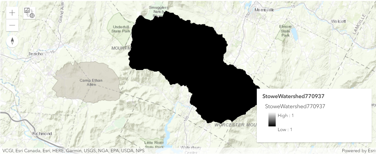
This watershed represents all of the area that flows to the specified outlet. The watershed comprises almost the entirety of Stowe's town boundaries, indicating that almost all rainfall that lands in Stowe will go rushing through the actual town, rather than draining away from it.
m9.add_layer(stowe_watershed)
m9.zoom_to_layer(stowe_watershed)
m9.legend = TrueYou've determined how water will flow throughout Stowe, Vermont. Based on your results, you snapped your outlet point to the location of the Little River in your DEM. From your flow direction layer and your outlet point, you determined the location of the watershed upstream of the town. Next, you'll use several of your hydrologic and elevation layers to determine how fast water will flow to the outlet point.
Create a velocity field
Previously, you created a watershed for the Stowe area, which you'll use as a study area for much of your subsequent analysis. Next, you'll start determining how long it takes water to reach the outlet, allowing the town to better predict when flooding will occur during a hypothetical rainfall event. To determine the time it takes water to flow somewhere, you first need to determine how fast water flows. You'll calculate the speed of flowing water with a velocity field, another type of raster layer. There are many types of velocity fields, and they can be calculated with a wide variety of mathematical equations. You'll create a velocity field that is spatially variant, but time and discharge invariant. This means that your velocity field satisfies the following assumptions:
- Velocity is affected by spatial components such as slope and flow - accumulation (spatially variant).
- Velocity at a given location does not change over time (time invariant).
- Velocity at a given location does not depend on the location's rate of water flow (discharge invariant).
In reality, velocity could be time variant and would definitely be discharge variant. However, incorporating these variants would require additional datasets that might not be available and use modeling techniques that might not be replicable in a GIS environment. The spatially variant, time- and discharge-invariant velocity field will provide a generally accurate result, although it's important to remember that any method will be only an approximation of observed phenomena.
You'll use a method for creating velocity fields first proposed by Maidment et al. (1996). In this method, each cell in the velocity field is assigned a velocity based on the local slope and the upstream contributing area (the number of cells that flow into that cell, or flow accumulation). They use the following equation:
V = $V_m$ * ($S^b$$A^c$) / ($S^b$$A^c$$_m$) ------------- (1)
Where V is the velocity of a single cell with a local slope of s and an upstream contributing area of A. Coefficients b and c can be determined by calibration, a statistical method of tweaking model parameters so that predicted data is as close as possible to observed data. In this scenario, you'll use the method's recommended value of b = c = 0.5. $V_m$ is the average velocity of all cells in the watershed. You'll assume an average velocity of $V_m$ = 0.1 m/s. Lastly, $S^b$$A^c$$_m$ is the average slope-area term throughout the watershed. To avoid results that are unrealistically fast or slow, you'll set limits for minimum and maximum velocities. The lower limit will be 0.02 meters per second, while the upper limit will be 2 meters per second.
This equation is only one of many ways that a velocity field can be calculated, and it comes with several assumptions and limitations of its own.
Create the slope raster
slope tool calculates slope value for each call of the given raster and creates a new raster layer with each cell representing th slope value corresponding to the original raster. The slope is determined by the change in elevation between cells, so it requires your original elevation layer as an input.
slope_type=2 represents the Percent rise measurement option which calculates slope as a percentage of vertical elevation over horizontal elevation, as opposed to a measurement in degrees. You'll leave the remaining parameters unchanged. The planar method is appropriate to use on local scale areas (small areas such as this watershed) where slope differences between planar and geodesic methods are minimal. The Z factor is only used if the units for measuring X and Y distance are different from the units for measuring Z (height) distance.
stowe_slope = slope(stowe_dem, z_factor=1, slope_type=2).save('stowe_slope' + str(dt.now().microsecond))m10 = gis.map('Stowe, Vermont')
m10
The darker colors represent steeper slope. While the mountain peaks tend to have the highest slopes, the stream bed, around which the town is located, have a relatively flat slope.
m10.add_layer(stowe_slope)m10.zoom_to_layer(stowe_slope)m10.legend = TrueCalculate the slope-area term
Now that you have a raster layer for both slope and flow accumulation area, you'll calculate a new raster layer that combines them. This layer will show the slope-area term (the value $S^b$$A^c$ from the Maidment et al. equation). raster_calculator tool allows you to create customized raster layers based on an equation that you specify.
SquareRoot("Stowe_slope") * SquareRoot("Stowe_flow_accumulation")
The reason you're finding the square root of the slope and flow accumulation is because you're using the recommended coefficients (b = c = 0.5) of Maidment et al. A coefficient of 0.5 is equivalent to the square root of the value.
stowe_slope_area_term = raster_calculator([stowe_slope.layers[0], stowe_flow_accumulation.layers[0]],
                                          input_names=['a','b'],
                                          expression='SquareRoot(a) * SquareRoot(b)').save('Stowe_slope_area_term' +
                                                                                           str(dt.now().microsecond))
Our study area is confined to the area occupied by the watershed, so we will mask stowe_slope_area_term layer in the shape of watershed.
masked_Stowe_slope_area_term = con([stowe_watershed.layers[0],
                                    stowe_slope_area_term.layers[0],
                                    0]).save('masked_Stowe_slope_area_term' +
                                             str(dt.now().microsecond))
m11 = gis.map('Stowe, Vermont')
m11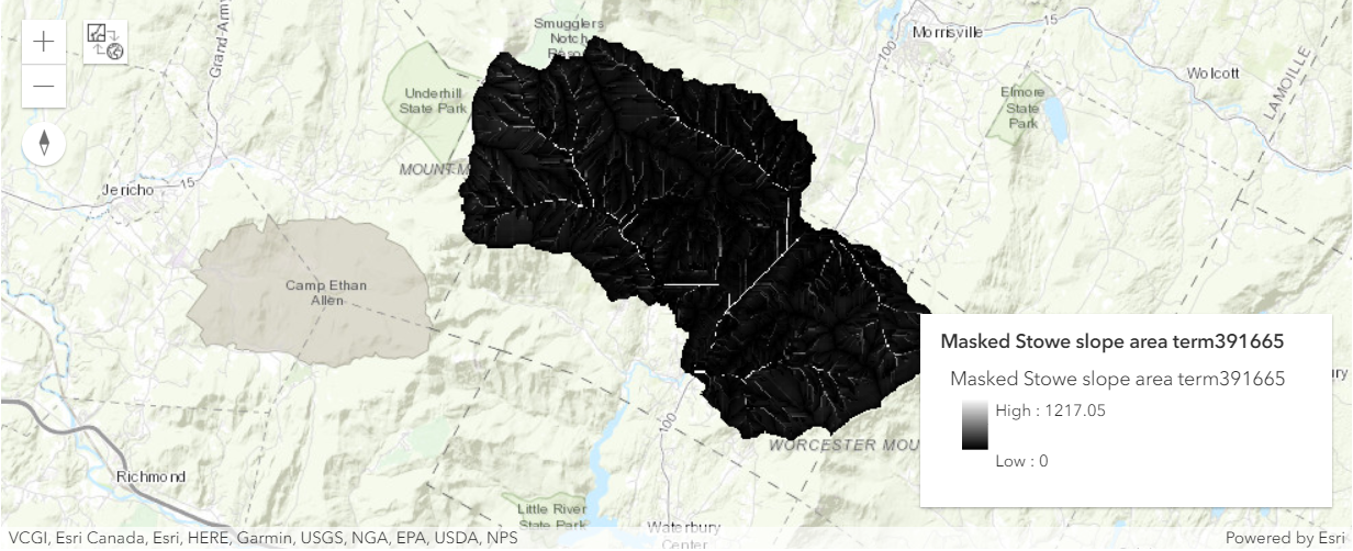
m11.add_layer(masked_Stowe_slope_area_term)m11.zoom_to_layer(masked_Stowe_slope_area_term)m11.legend = TrueCalculate the velocity field
Now that you have the slope-area term, you can calculate a velocity field using the following equation:
V = $V_m$ ($S^b$$A^c$) / ($S^b$$A^c$$_m$) ------------- (1)
As mentioned previously, $V_m$ is the average velocity of all cells in the watershed. You'll use an assumed average value of $V_m$ = 0.1, which is recommended by Maidment et al. Similarly, $S^b$$A^c$$_m$ is the average slope-area term across the watershed. Because you've calculated slope-area term for the watershed, you can determine the exact average rather than relying on an assumed value.
masked_Stowe_slope_area_term.layers[0].properties{
"currentVersion": 10.8,
"serviceDescription": "Hosted/masked_Stowe_slope_area_term391665",
"name": "Hosted/masked_Stowe_slope_area_term391665",
"description": "",
"extent": {
"xmin": 471060.08257249475,
"ymin": 208312.35339681862,
"xmax": 494700.08257249475,
"ymax": 231352.35339681862,
"spatialReference": {
"wkt": "PROJCS[\"NAD_1983_Transverse_Mercator\",GEOGCS[\"GCS_North_American_1983\",DATUM[\"D_North_American_1983\",SPHEROID[\"GRS_1980\",6378137.0,298.257222101]],PRIMEM[\"Greenwich\",0.0],UNIT[\"Degree\",0.0174532925199433]],PROJECTION[\"Transverse_Mercator\"],PARAMETER[\"False_Easting\",500000.0],PARAMETER[\"False_Northing\",0.0],PARAMETER[\"Central_Meridian\",-72.5],PARAMETER[\"Scale_Factor\",0.999964286],PARAMETER[\"Latitude_Of_Origin\",42.5],UNIT[\"Meter\",1.0]]"
}
},
"initialExtent": {
"xmin": 471060.08257249475,
"ymin": 208312.35339681862,
"xmax": 494700.08257249475,
"ymax": 231352.35339681862,
"spatialReference": {
"wkt": "PROJCS[\"NAD_1983_Transverse_Mercator\",GEOGCS[\"GCS_North_American_1983\",DATUM[\"D_North_American_1983\",SPHEROID[\"GRS_1980\",6378137.0,298.257222101]],PRIMEM[\"Greenwich\",0.0],UNIT[\"Degree\",0.0174532925199433]],PROJECTION[\"Transverse_Mercator\"],PARAMETER[\"False_Easting\",500000.0],PARAMETER[\"False_Northing\",0.0],PARAMETER[\"Central_Meridian\",-72.5],PARAMETER[\"Scale_Factor\",0.999964286],PARAMETER[\"Latitude_Of_Origin\",42.5],UNIT[\"Meter\",1.0]]"
}
},
"fullExtent": {
"xmin": 471060.08257249475,
"ymin": 208312.35339681862,
"xmax": 494700.08257249475,
"ymax": 231352.35339681862,
"spatialReference": {
"wkt": "PROJCS[\"NAD_1983_Transverse_Mercator\",GEOGCS[\"GCS_North_American_1983\",DATUM[\"D_North_American_1983\",SPHEROID[\"GRS_1980\",6378137.0,298.257222101]],PRIMEM[\"Greenwich\",0.0],UNIT[\"Degree\",0.0174532925199433]],PROJECTION[\"Transverse_Mercator\"],PARAMETER[\"False_Easting\",500000.0],PARAMETER[\"False_Northing\",0.0],PARAMETER[\"Central_Meridian\",-72.5],PARAMETER[\"Scale_Factor\",0.999964286],PARAMETER[\"Latitude_Of_Origin\",42.5],UNIT[\"Meter\",1.0]]"
}
},
"pixelSizeX": 30,
"pixelSizeY": 30,
"bandCount": 1,
"pixelType": "F32",
"minPixelSize": 0,
"maxPixelSize": 0,
"copyrightText": "",
"serviceDataType": "esriImageServiceDataTypeGeneric",
"minValues": [
0
],
"maxValues": [
1217.0540771484375
],
"meanValues": [
15.97043191494731
],
"stdvValues": [
37.085463797614466
],
"objectIdField": "",
"fields": [],
"capabilities": "Image, Metadata",
"defaultMosaicMethod": "Center",
"allowedMosaicMethods": "",
"sortField": "",
"sortValue": null,
"sortAscending": true,
"mosaicOperator": "First",
"defaultCompressionQuality": 75,
"defaultResamplingMethod": "Nearest",
"maxImageHeight": 4100,
"maxImageWidth": 15000,
"allowRasterFunction": true,
"rasterFunctionInfos": [
{
"name": "None",
"description": "",
"help": ""
}
],
"rasterTypeInfos": [
{
"name": "Raster Dataset",
"description": "Supports all ArcGIS Raster Datasets",
"help": ""
}
],
"mensurationCapabilities": "Basic",
"hasHistograms": true,
"hasColormap": false,
"hasRasterAttributeTable": false,
"minScale": 0,
"maxScale": 0,
"exportTilesAllowed": false,
"hasMultidimensions": false,
"supportsStatistics": false,
"supportsAdvancedQueries": false,
"editFieldsInfo": null,
"ownershipBasedAccessControlForRasters": null,
"allowComputeTiePoints": false,
"useStandardizedQueries": true,
"advancedQueryCapabilities": {
"useStandardizedQueries": true,
"supportsStatistics": false,
"supportsOrderBy": false,
"supportsDistinct": false,
"supportsPagination": false
},
"spatialReference": {
"wkt": "PROJCS[\"NAD_1983_Transverse_Mercator\",GEOGCS[\"GCS_North_American_1983\",DATUM[\"D_North_American_1983\",SPHEROID[\"GRS_1980\",6378137.0,298.257222101]],PRIMEM[\"Greenwich\",0.0],UNIT[\"Degree\",0.0174532925199433]],PROJECTION[\"Transverse_Mercator\"],PARAMETER[\"False_Easting\",500000.0],PARAMETER[\"False_Northing\",0.0],PARAMETER[\"Central_Meridian\",-72.5],PARAMETER[\"Scale_Factor\",0.999964286],PARAMETER[\"Latitude_Of_Origin\",42.5],UNIT[\"Meter\",1.0]]"
}
}masked_Stowe_slope_area_term.layers[0].properties['maxValues'][0]1217.0540771484375
masked_Stowe_slope_area_term.layers[0].properties['meanValues'][0]15.97043191494731
stowe_velocity_unlimited = raster_calculator([masked_Stowe_slope_area_term.layers[0]],
                                          input_names=['Stowe_slope_area_term'],
                                          expression='0.1 * (Stowe_slope_area_term/15.97043191494731)'
                                            ).save('Stowe_velocity_unlimited' + str(dt.now().microsecond))
m12 = gis.map('Stowe, Vermont')
m12
m12.add_layer(stowe_velocity_unlimited)m12.zoom_to_layer(stowe_velocity_unlimited)m12.legend = TrueLimit the velocities
The raster layer you created is a velocity field, but it has unrealistically high and low velocities. For instance, some values in the field have a velocity of 0 meters per second, which is unlikely during an extreme rainfall event. Likewise, the maximum value of approximately 7.5 meters per second is unrealistic even during a major flood. You'll limit the velocity values with a lower limit of 0.02 meters per second and an upper limit of 2 meters per second.
from arcgis.raster.functions import greater_than_equal, less_than_equalexpression = greater_than_equal([stowe_velocity_unlimited.layers[0], 0.02])lower_limited_velocity = con([expression,
stowe_velocity_unlimited.layers[0],
0.02]).save('lower_limited_velocity' + str(dt.now().microsecond))expression = less_than_equal([stowe_velocity_unlimited.layers[0], 2])stowe_velocity = con([expression,
lower_limited_velocity.layers[0],
2]).save('stowe_velocity' + str(dt.now().microsecond))m13 = gis.map('Stowe, Vermont')
m13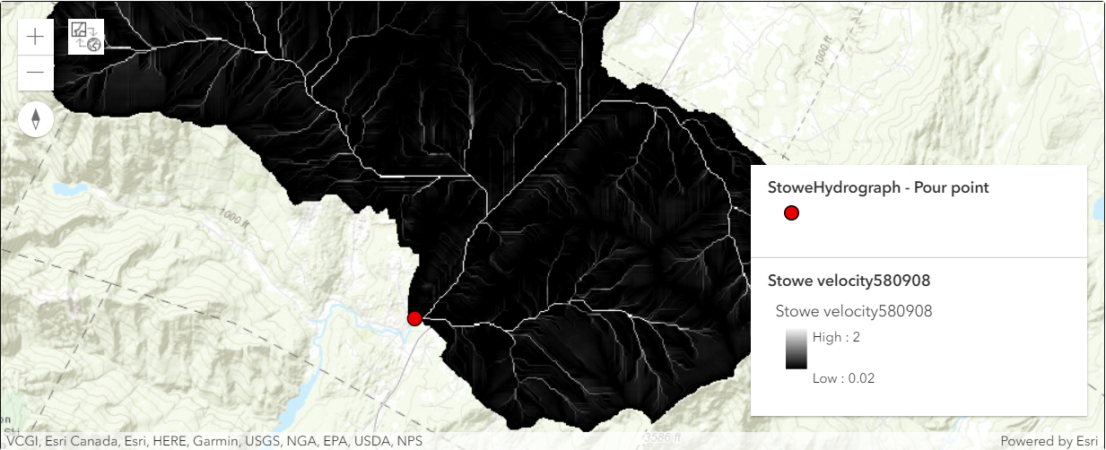
In this map, darker colors represent a slower velocity, while lighter colors represent a faster velocity. Water tends to flow fastest in streams, where the largest amount of water has accumulated. The area around Stowe is no exception, indicating that water will flow at its fastest when funneling toward the outlet point downstream of the town.
m13.add_layer(stowe_velocity)m13.add_layer(pour_point)m13.zoom_to_layer(stowe_velocity)m13.legend = TrueYou've derived a spatially variant, time- and discharge-invariant velocity field from flow accumulation and slope raster layers. You used one of many formulas that can calculate velocity fields to do so. Now that you know how fast water is flowing through Stowe during your hypothetical rainfall event, you'll determine how long it takes water to flow to the outlet.
Create an isochrone map
Previously, you used your flow accumulation and watershed layers to create a velocity field that predicts how fast water will flow throughout Stowe, Vermont. Your velocity field showed that water will move fastest along the streams leading through town, but you still can't create a unit hydrograph because you don't know the time it will take water to flood to your outlet point. Next, you'll create an isochrone map, which maps the time it takes to reach a specified location from anywhere else in an area. To create the isochrone map, you'll first create a weight grid. Then, you'll assess the time it takes for water to reach the outlet and reclassify those times into isochrone zones.
Create a weight grid
Flow time is calculated with a relatively simple equation: The length that water must flow divided by the speed at which it flows. While you know how fast water flows due to your velocity field, you don't know flow length. To determine flow length, you need two variables: flow direction (which you know) and weight (which you don't). Weight, in regard to flow, represents impedance. For instance, water flowing through forested land takes longer than water flowing over smooth rock because it's impeded by terrain. While calculating weight may seem difficult without detailed terrain data, you can derive an equation to calculate it based on the following two equations for finding flow time:
Flow time [T] = Flow Length [L] / Velocity $LT^{-1}$
Flow time [T] = Flow Length [L] * Weight $L^{-1}T$
By combining these equations, you get a new equation:
Weight [$L^{-1}T$] = 1 / Velocity $LT^{-1}$
Thus, you can determine weight using your velocity field layer. Later, you'll use your weight grid layer in conjunction with your flow direction layer to determine flow length and flow time.
stowe_weight = raster_calculator([stowe_velocity.layers[0]],
                                          input_names=['stowe_velocity'],
                                          expression='1 / stowe_velocity').save('Stowe_weight' +
                                                                                str(dt.now().microsecond))
m14 = gis.map('Stowe, Vermont')
m14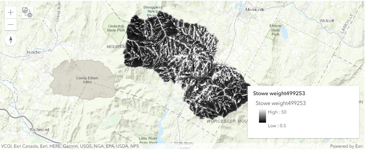
m14.add_layer(stowe_weight)
m14.zoom_to_layer(stowe_weight)
m14.legend = True
You created the flow direction layer before you determined the Stowe watershed, so the layer's extent covers far more than your area of interest. You'll extract a new version of the flow direction layer that only covers the watershed.
We will use con tool to clip a raster layer to a certain extent based on the extent of another layer.
stowe_watershed_flow_dir = con([stowe_watershed.layers[0],
                                stowe_fill_flow_direction.layers[0],
                                0]).save('stowe_watershed_flow_dir' + str(dt.now().microsecond))
from arcgis.raster.functions import colormap, stretch
stowe_watershed_flow_dir_colormap = colormap(stowe_watershed_flow_dir.layers[0], colormap_name="Random")m15 = gis.map('Stowe, Vermont')
m15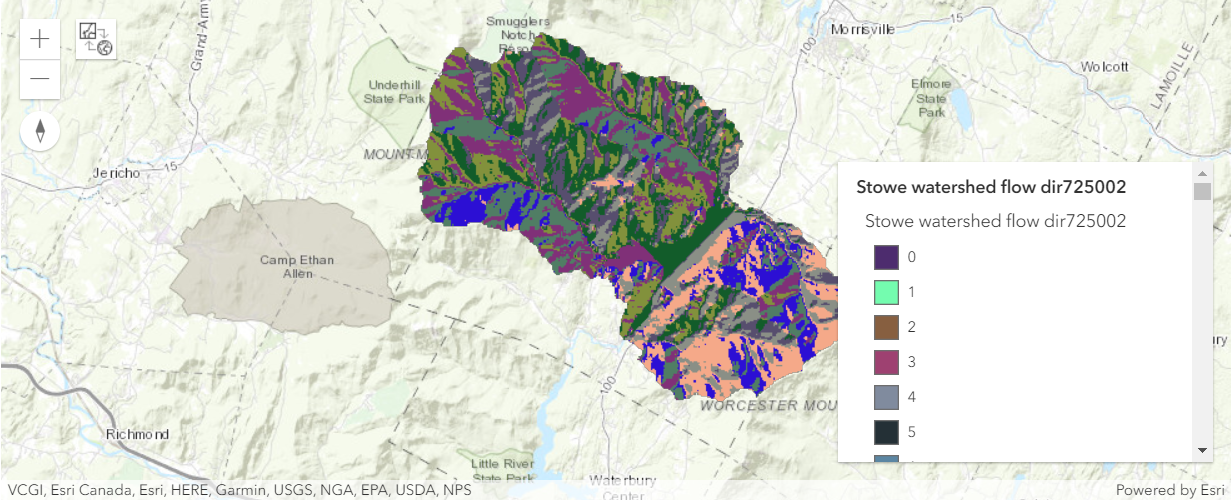
m15.add_layer(stowe_watershed_flow_dir_colormap)m15.zoom_to_layer(stowe_watershed_flow_dir_colormap)m15.legend = TrueAccess flow time to outlet pour point
Finally you have gathered all layers needed to determine flow time, and the next step of the task would require you to use the flow_length tool. While this tool, as its name suggests, normally calculates flow length, it has an optional parameter to include a weight raster and whenever a weight raster is included, the tool then calculates flow time instead.
from arcgis.raster.functions.gbl import flow_lengthstowe_time = flow_length(input_flow_direction_raster=stowe_watershed_flow_dir.layers[0],
input_weight_raster=stowe_weight.layers[0]).save('stowe_time' + str(dt.now().microsecond))Each cell in this raster layer contains a value that represents the time in seconds for water to flow to the outlet from the cell. Darker colors represent shorter flow times. Water takes the least amount of time to flow from the low-lying stream beds closest to the outlet, while water falling in the western mountains takes longer.
m16 = gis.map('Stowe, Vermont')
m16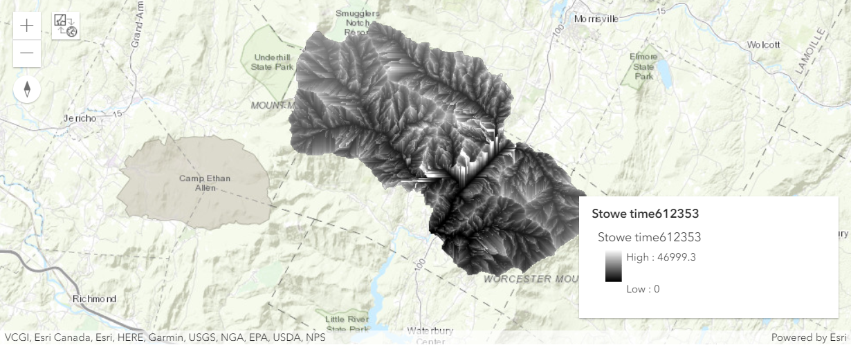
The time it takes for water to flow to the outlet ranges from 0 seconds (rain that falls on the outlet itself) to about 47,000 seconds—over 13 hours!
m16.add_layer(stowe_time)m16.zoom_to_layer(stowe_time)m16.legend = TrueReclassify flow time into isochrone zones
Your flow time raster layer contains an extremely high number of unique values, which will make subsequent analysis complicated and unwieldy. To make things easier, you'll reclassify the flow time layer into isochrone zones.
An isochrone is a contour line that passes through points of roughly equal travel time to the outlet of the watershed. You'll define isochrones at equal time intervals of 1,800 seconds (or 30 minutes). For larger areas, isochrones can use different intervals, but for the Stowe watershed, this time interval should be appropriate. With this time interval, every cell in the first isochrone zone will take about 1,800 seconds to reach the outlet, every cell in the second isochrone zone will take about 3600 seconds, and so on. You'll later use these time intervals as the ordinate in your unit hydrograph.
You'll use remap tool to classify flow time values that fall between a specific range of values (say, 0 and 1,800 or 1,800 to 3,600) to the upper limit of the range. Thus, a value of 907 would be reclassified to 1,800, while a value of 2,145 would be reclassified to 3,600.
from arcgis.raster.functions import remapinput_range = []
output = []
for i in range(0, 47000, 1800):
input_range.append(i)
input_range.append(i + 1800)
output.append(i + 1800)stowe_isochrones = remap(stowe_time.layers[0],
input_ranges=input_range,
output_values=output).save('stowe_isochrones' + str(dt.now().microsecond))hist = stowe_isochrones.layers[0].histogramscount = hist[0]['counts']counts = [i for i in count if i != 0]counts[673, 2889, 6107, 11924, 18738, 24368, 27925, 28176, 24156, 16865, 10194, 5411, 2670, 1309, 665, 346, 233, 176, 119, 80, 52, 36, 23, 13, 10, 3, 1]
import pandas as pdtable = pd.DataFrame()table['Time(seconds)'] = outputtable['counts'] = countstable| range | Time(seconds) | counts | |
|---|---|---|---|
| 0 | 1800 | 1800 | 673 |
| 1 | 3600 | 3600 | 2889 |
| 2 | 5400 | 5400 | 6107 |
| 3 | 7200 | 7200 | 11924 |
| 4 | 9000 | 9000 | 18738 |
| 5 | 10800 | 10800 | 24368 |
| 6 | 12600 | 12600 | 27925 |
| 7 | 14400 | 14400 | 28176 |
| 8 | 16200 | 16200 | 24156 |
| 9 | 18000 | 18000 | 16865 |
| 10 | 19800 | 19800 | 10194 |
| 11 | 21600 | 21600 | 5411 |
| 12 | 23400 | 23400 | 2670 |
| 13 | 25200 | 25200 | 1309 |
| 14 | 27000 | 27000 | 665 |
| 15 | 28800 | 28800 | 346 |
| 16 | 30600 | 30600 | 233 |
| 17 | 32400 | 32400 | 176 |
| 18 | 34200 | 34200 | 119 |
| 19 | 36000 | 36000 | 80 |
| 20 | 37800 | 37800 | 52 |
| 21 | 39600 | 39600 | 36 |
| 22 | 41400 | 41400 | 23 |
| 23 | 43200 | 43200 | 13 |
| 24 | 45000 | 45000 | 10 |
| 25 | 46800 | 46800 | 3 |
| 26 | 48600 | 48600 | 1 |
You've used your velocity field raster layer to create a weight grid. This weight grid represented impedance to downstream flow and helped you create a flow time raster layer. You also reclassified flow times into 27 isochrones with an equal interval time of 1,800 seconds. Next, you'll develop a time-discharge relationship at the outlet for unit excess rainfall that occurs uniformly, over the entire watershed, in intervals of 1,800 seconds. Finally, you'll plot this relationship to create your unit hydrograph.
Create a unit hydrograph
Now, you'll calculate area to show relationship between time and the area of water flowing into the outlet. Then, you'll use this table to plot a unit hydrograph that will show the times at which the most water flows into the outlet, allowing for better flood prediction in future rainfall events.
table['area'] = table['counts']*30*30table['area'] = table['area']/1800table| range | Time(seconds) | counts | area | |
|---|---|---|---|---|
| 0 | 1800 | 1800 | 673 | 336.5 |
| 1 | 3600 | 3600 | 2889 | 1444.5 |
| 2 | 5400 | 5400 | 6107 | 3053.5 |
| 3 | 7200 | 7200 | 11924 | 5962.0 |
| 4 | 9000 | 9000 | 18738 | 9369.0 |
| 5 | 10800 | 10800 | 24368 | 12184.0 |
| 6 | 12600 | 12600 | 27925 | 13962.5 |
| 7 | 14400 | 14400 | 28176 | 14088.0 |
| 8 | 16200 | 16200 | 24156 | 12078.0 |
| 9 | 18000 | 18000 | 16865 | 8432.5 |
| 10 | 19800 | 19800 | 10194 | 5097.0 |
| 11 | 21600 | 21600 | 5411 | 2705.5 |
| 12 | 23400 | 23400 | 2670 | 1335.0 |
| 13 | 25200 | 25200 | 1309 | 654.5 |
| 14 | 27000 | 27000 | 665 | 332.5 |
| 15 | 28800 | 28800 | 346 | 173.0 |
| 16 | 30600 | 30600 | 233 | 116.5 |
| 17 | 32400 | 32400 | 176 | 88.0 |
| 18 | 34200 | 34200 | 119 | 59.5 |
| 19 | 36000 | 36000 | 80 | 40.0 |
| 20 | 37800 | 37800 | 52 | 26.0 |
| 21 | 39600 | 39600 | 36 | 18.0 |
| 22 | 41400 | 41400 | 23 | 11.5 |
| 23 | 43200 | 43200 | 13 | 6.5 |
| 24 | 45000 | 45000 | 10 | 5.0 |
| 25 | 46800 | 46800 | 3 | 1.5 |
| 26 | 48600 | 48600 | 1 | 0.5 |
%matplotlib inline
import matplotlib.pyplot as plt

hydrograph_plot = table.plot('Time(seconds)', 'area', title="Unit Hydrograaph as Outlet Point", grid=True, figsize=(10, 8))
hydrograph_plot.set_xlabel("Time(seconds)")
hydrograph_plot.set_ylabel("Discharge of outlet per unit excess rainfall(sq. meters per second)")
plt.show()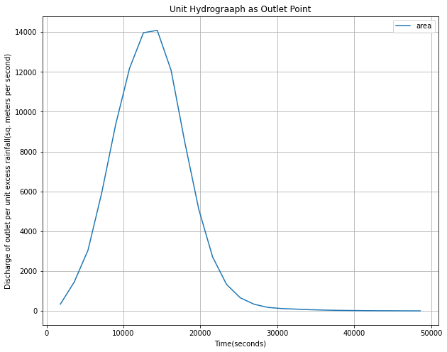
The above plot shows when water discharge at the outlet is at its height during a predicted rainfall event.
Conclusion
In this notebook, we have gained knowledege about various tools available in arcgis.raster.functions and arcgis.raster.functions.gbl module in order to predict floods using unit hydrographs in order to plan for and respond to flood events more effectively.
Acknowledgements
Data acquired from the Vermont Center for Geographic Information (VCGI), the NHDPlus Version 2 dataset, and the United States Geological Survey (USGS).
