Introduction
We can use multispectral imagery to train any arcgis.learn model that works with imagery. Apart from the standard workflow to train a arcgis.learn model there are a few additional parameters that can be used while working with multispectral imagery. In this guide we would discuss these additional parameters.
Prerequisites
- To work with multispectral data gdal needs to be installed in addition to fastai and pytorch, please refer to the section "Install deep learning dependencies of arcgis.learn module" on this page for detailed documentation on installation of these dependencies.
Imports
import arcgis
from arcgis.learn import prepare_data, UnetClassifier
Data preparation
While working with multispectral data we can use the following keyword arguments in addition to the standard parameters for the prepare_data() function.
-
Right now multispectral workflow is used for the dataset in the following mutually exclusive cases:
- If the imagery source is not having exactly three bands
- If there is any band other than RGB in the imagery source
- Incase of three band iamgery all bands in the imagery source are having well known names.
- Any of these keyword arguments is sepcified
imagery_type,bands,rgb_bands.
-
imagery_type: The type of imagery used to export the training data. We can use any of the well know imagery types:- 'sentinel2'
- 'naip'
- 'landsat8'
- 'ms' - any other type of imagery
If the imagery used to export the training data is not one of the well know types, you can specify 'ms' against
imagery_type. In that case we need to either specifyrgb_bandsorbandsparameter to preserve weights for the RGB bands otherwise all the bands would be considered unknown. -
bands: If training data is not exported using one of the well known imagery type, we can specify the bands contained in our imagery. For example, ['r', 'g', 'b', 'nir', 'u'] here 'nir' is and 'u' is a miscellaneous band.
rgb_bands: We can specify the indices of red, green, blue bands in the imagery or None if that band does not exist in the imagery. This is further used as the default band combination for visualization using the{data}.show_batch()and{model}.show_results()methods, this is an optional parameter. For example, [2, 1, 0] or [2, 1, None].extract_bands: By default the model gets trained on all bands available in the imagery of our training data. We can use this parameter to filter the bands on which we want to train our model on. For example '[4, 2, 1, 0]' if we do not want to train on the band at 3 index of the imagery.norm_pct: The percentage of training data used to calculate imagery statistics which is further used to normalize the data while training the model. It is an optional parameter and by default it is set to 0.3 or 30% of data.
data = prepare_data(
    r'C:\Workspace\Data\LULC\traindata_sentinel2_ms_400px',
    batch_size=4,
    imagery_type='sentinel2',
    norm_pct=1
)
Visualize Training data
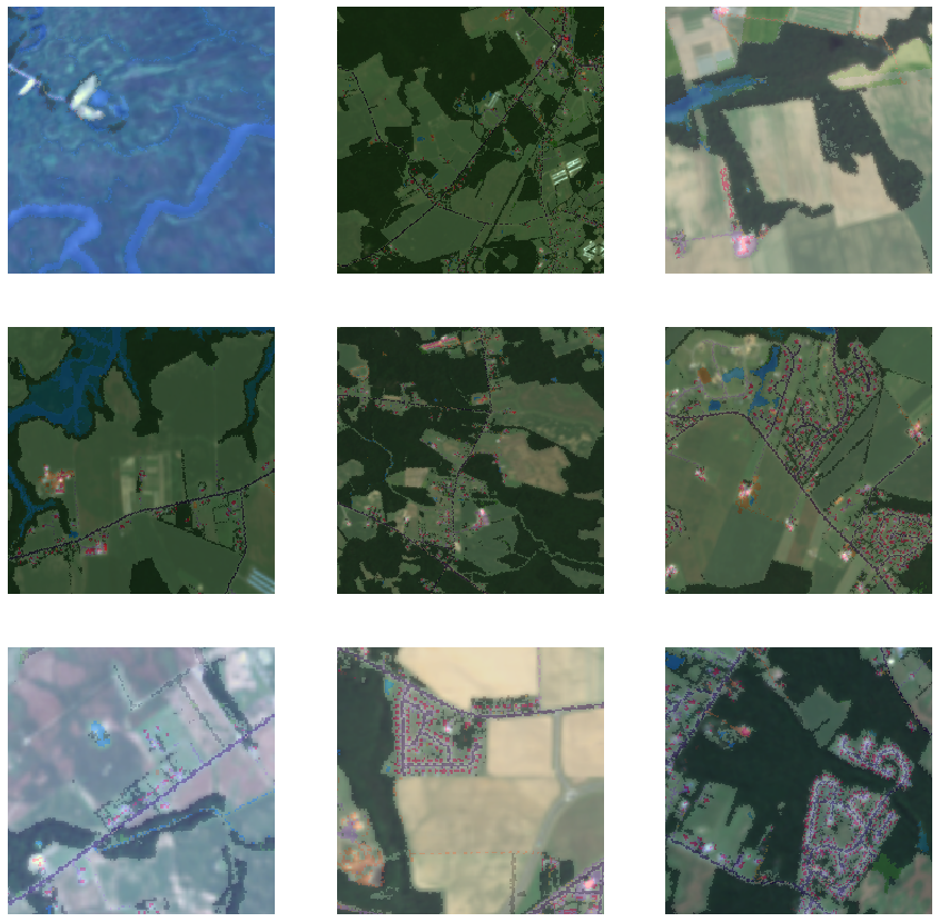
we can use the {data}.show_batch() method to visualize a few samples of the training data. Following parameters can be used with multispectral imagery to control the visualization.
rgb_bands: The band combination in which we want to visualize our training data, For example [2, 1, 0] or ['nir', 'green', 'blue'].stretch_type: The type of stretching we want to apply to imagery in our training data for visualization.- 'minmax' - Default! This stretches each image chips by min-max values.
- 'percentclip' - This stretched image chips by clipping histogram by .25%.
statistics_type: The type of stretching we want to apply to imagery in our training data for visualization.- 'dataset' - Default! This stretches each image chip using global statistics.
- 'DRA' - stands for Dynamic Range Adjustment. This stretches each image chip using its individual statistics.
data.show_batch(statistics_type='DRA', alpha=0.5)
Different Band Combination
False Color Composite
red -> nir
green -> green
blue -> blue
data.show_batch(rgb_bands=[7, 2, 1], statistics_type='DRA', alpha=0.5)
Train Model
Model Initialization options
arcgis.learn uses transfer learning to enhance the model training experience. To train these models with multispectral data the model needs to accommodate the various types of bands available in multispectral imageries.
This is done by re-initializing the first layer of the model, an ArcGIS environment variable arcgis.env.type_init_tail_parameters can be used to specify the scheme in which the weights are initialized for the layer. Valid weight initialization schemes are:
- 'random' - default: Random weights are initialized for Non-RGB bands while preserving pretrained weights for RGB bands.
- 'red_band': Weights corresponding to the Red band from the pretrained model's layer are cloned for Non-RGB bands while preserving pretrained weights for RGB bands.
- 'all_random': Random weights are initialized for RGB bands as well as Non-RGB bands.
arcgis.env.type_init_tail_parameters = 'red_band'# Create the model
model = UnetClassifier(data)Learning Rate
# Find a learning rate
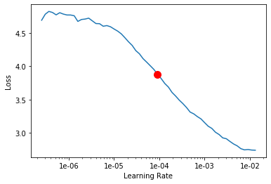
model.lr_find()
9.120108393559096e-05
We can use the {data}.lr_find() method to find an appropriate learning rate. Because the first layer of the model has been reinitalized it is trainable and must be trained at a lower learning rate then the remaining trainable part of the model. To do that we can use the slice(low_lr:high_lr) notation, specifying a lower learning rate for the first layer and a higher learning rate for the remaining trainable part of the model.
Because the first layer in our model has been just initialized, we might need to train the model a bit longer to get the best results.
model.fit(50, lr=slice(0.00001, 0.001), checkpoint=False)| epoch | train_loss | valid_loss | accuracy | time |
|---|---|---|---|---|
| 0 | 3.136030 | 1.573169 | 0.399334 | 00:17 |
| 1 | 2.458116 | 1.229420 | 0.572054 | 00:07 |
| 2 | 2.122384 | 1.320223 | 0.538070 | 00:07 |
| 3 | 1.906248 | 1.412342 | 0.399163 | 00:07 |
| 4 | 1.742509 | 1.021113 | 0.633614 | 00:07 |
| 5 | 1.603904 | 1.058293 | 0.613756 | 00:08 |
| 6 | 1.514009 | 0.939518 | 0.722907 | 00:10 |
| 7 | 1.488245 | 0.993276 | 0.712157 | 00:09 |
| 8 | 1.429352 | 0.977122 | 0.694898 | 00:09 |
| 9 | 1.355745 | 0.995815 | 0.675849 | 00:09 |
| 10 | 1.319153 | 1.073880 | 0.624833 | 00:08 |
| 11 | 1.288624 | 0.920015 | 0.652575 | 00:08 |
| 12 | 1.240515 | 0.861558 | 0.736591 | 00:08 |
| 13 | 1.227835 | 1.010466 | 0.656342 | 00:09 |
| 14 | 1.254720 | 1.209687 | 0.691024 | 00:09 |
| 15 | 1.254659 | 0.977635 | 0.745141 | 00:08 |
| 16 | 1.226321 | 0.899011 | 0.752523 | 00:08 |
| 17 | 1.198589 | 1.078376 | 0.677117 | 00:08 |
| 18 | 1.177784 | 0.797890 | 0.752160 | 00:08 |
| 19 | 1.139314 | 0.822118 | 0.771377 | 00:08 |
| 20 | 1.121551 | 0.847090 | 0.747106 | 00:08 |
| 21 | 1.099947 | 0.789873 | 0.755979 | 00:08 |
| 22 | 1.088178 | 0.891662 | 0.758869 | 00:08 |
| 23 | 1.066239 | 0.835028 | 0.748131 | 00:09 |
| 24 | 1.047243 | 0.778206 | 0.768240 | 00:08 |
| 25 | 1.007829 | 0.716469 | 0.786926 | 00:08 |
| 26 | 0.978055 | 0.757787 | 0.763919 | 00:08 |
| 27 | 0.961286 | 0.798902 | 0.763716 | 00:08 |
| 28 | 0.948301 | 0.718838 | 0.779050 | 00:08 |
| 29 | 0.938797 | 0.725577 | 0.793834 | 00:08 |
| 30 | 0.929100 | 0.760337 | 0.757442 | 00:08 |
| 31 | 0.912958 | 0.719378 | 0.786783 | 00:08 |
| 32 | 0.899271 | 0.670808 | 0.807665 | 00:08 |
| 33 | 0.893611 | 0.710234 | 0.793507 | 00:08 |
| 34 | 0.880450 | 0.681021 | 0.802778 | 00:08 |
| 35 | 0.871665 | 0.666591 | 0.805692 | 00:08 |
| 36 | 0.867548 | 0.683682 | 0.800163 | 00:08 |
| 37 | 0.869506 | 0.682281 | 0.808909 | 00:08 |
| 38 | 0.862610 | 0.699594 | 0.796847 | 00:08 |
| 39 | 0.851020 | 0.676894 | 0.799326 | 00:08 |
| 40 | 0.836587 | 0.662309 | 0.804034 | 00:08 |
| 41 | 0.823378 | 0.657619 | 0.807681 | 00:08 |
| 42 | 0.806154 | 0.651746 | 0.812133 | 00:08 |
| 43 | 0.820973 | 0.655077 | 0.810647 | 00:08 |
| 44 | 0.815987 | 0.658856 | 0.806657 | 00:08 |
| 45 | 0.815662 | 0.656755 | 0.807761 | 00:08 |
| 46 | 0.812138 | 0.650601 | 0.809953 | 00:08 |
| 47 | 0.808693 | 0.647900 | 0.811683 | 00:08 |
| 48 | 0.810618 | 0.656571 | 0.807753 | 00:08 |
| 49 | 0.795867 | 0.657882 | 0.806724 | 00:08 |
Validate results
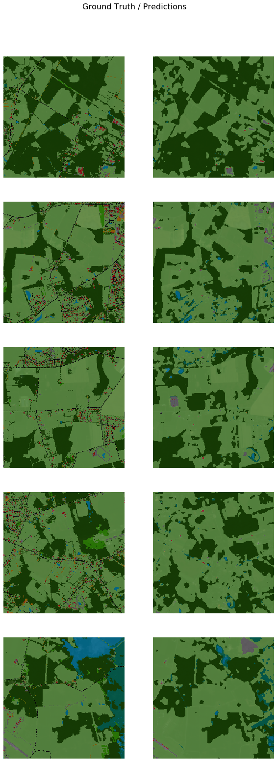
we can use the {model}.show_results() method to validate a few predictions from the validation dataset and compare them with the ground truth. Following parameters can be used with multispectral imagery to control the visualization.
rgb_bands: The band combination in which we want to visualize our training data, For example [2, 1, 0] or ['nir', 'green', 'blue'].stretch_type: The type of stretching we want to apply to imagery in our training data for visualization.- 'minmax' - Default! This stretches each image chips by min-max values.
- 'percentclip' - This stretched image chips by clipping histogram by .25%.
statistics_type: The type of stretching we want to apply to imagery in our training data for visualization.- 'dataset' - Default! This stretches each image chip using global statistics.
- 'DRA' - stands for Dynamic Range Adjustment. This stretches each image chip using its individual statistics.
model.show_results()
Inferencing
We can save the model using the {model}.save() method, output of this method is a saved model file in '.dlpk' format. The model can be then deployed using ArcGIS Pro or ArcGIS Image Server. Depending on the type of model which we train, some of the tools that work with these deep learning models are:
- Classify Pixels Using Deep Learning
- Detect Objects Using Deep Learning
- Classify Objects Using Deep Learning
In this example we have trained a UnetClassifier which is a pixel classification model, so the tool Classify Pixels Using Deep Learning would work with our saved model.
model.save('50e')WindowsPath('C:/Workspace/Data/LULC/traindata_sentinel2_ms_400px/models/50e')