- Data Science
- Deep Learning and Panoptic Segmentation
Introduction
Land cover classification is one of the most common tasks in remote sensing. It can have multiple applications and can be very useful in understanding an area, its geography, landscape, demographic, and more. Landcover classification can be further combined with building footprint extraction and object detection for even more detailed analysis. Currently, this is achieved through multiple models. However, using Panoptic Segmentation, we can detect objects of interest and also classify the pixels of a raster using a single model.
Panoptic Segmentation works with both types of classes - stuff and things. In deep learning jargon, stuff refers to the class that is indistinctive and uncountable, for example, vegetation, road, water, sky, etc. Most of the land cover classes will classify as stuff. Things refers to classes that are distinctive, for example, buildings, cars, pools, solar panels, etc., and are also referred to as instance classes.
Panoptic Segmentation models use three inputs during training - a raster, a feature layer or a classified raster that classifies each pixel in the raster into individual classes, and a feature layer containing polygons for the objects of interest (the instance classes). This notebook demonstrates how to use the Panoptic Segmentation model MaXDeepLab to classify Land Use Land Cover (LULC) and extract building footprints and cars using very high-resolution satellite imagery of Los Angeles County. The model has been trained using the ArcGIS Python API. The trained model can then be deployed in ArcGIS Pro or ArcGIS Enterprise to classify LULC and extract building footprints and cars.
Export training data
# Connect to GIS
from arcgis.gis import GIS
gis = GIS("home")
gis_ent = GIS('https://pythonapi.playground.esri.com/portal/')
The following imagery layer contains very high resolution imagery of a part of LA County in California. The spatial resolution of the imagery is 7.5 cm (4 inches), and it contains 3 bands: Red, Green, and Blue. It is used as the 'Input Raster' for exporting the training data.
training_raster = gis_ent.content.get('b405b34eb7d542deb4533fb80e925f6b')
training_rasterTo export training data for panoptic segmentation, we need two input layers. 1. A feature class or a classified raster for pixel classification. 2. A feature class with polygons for the instance classes to be detected.
The following feature layer contains the polygons for the LULC classes for the corresponding imagery of LA County. It is used as the 'Input Feature Class' for exporting the training data.
input_feature_class = gis.content.get('d64f11aea3ae47c19084f21c204ba318')
input_feature_classThe following feature layer contains the polygons for the building footprints and cars and will be used as the 'Instance Feature Class' for exporting the training data.
instance_feature_class = gis.content.get('22b83520db8f42ea98a5279b71684afd')
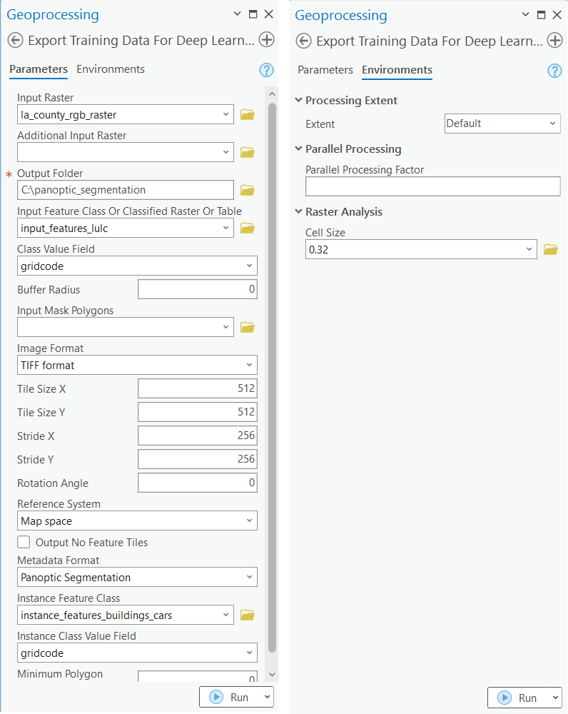
instance_feature_classTraining data can be exported by using the Export Training Data For Deep Learning tool available in ArcGIS Pro and ArcGIS Enterprise. For this example, we prepared the training data in ArcGIS Pro in the Panoptic Segmentation format using a chip_size of 512px and a cell_size of 0.32 ft. The Input Raster, the Input Feature Class and the Instance Feature Class have been made available to export the required training data. We have also provided a subset of the exported training data in the next section, if you want to skip this step.
Train the model
Necessary imports
%matplotlib inlineimport os
import zipfile
from pathlib import Path
from arcgis.learn import prepare_data, MaXDeepLabGet training data
We have already exported a smaller dataset and made it available so that it can be used by following the steps below. Exporting a larger dataset is suggested for better results.
training_data = gis.content.get('69544aca740d42d3a3e36f7ad5ddb485')
training_datafilepath = training_data.download(file_name=training_data.name)import zipfile
with zipfile.ZipFile(filepath, 'r') as zip_ref:
zip_ref.extractall(Path(filepath).parent)data_path = Path(os.path.join(os.path.splitext(filepath)[0]))Prepare data
We will specify the path to our training data and a few hyperparameters.
data_path: path of the folder/list of folders containing training data.batch_size: Number of images your model will train on each step inside an epoch. Depends on the memory of your graphic card.chip_size: The same as the tile size used while exporting the dataset. A smaller chip_size crops the tile.n_mask: The maximum number of masks, i.e., the sum of unique instances of all things classes and total stuff classes, in a chip. The default value is 30. You can increase it if there are many objects in a single chip. A warning message will be displayed in some of the methods if then_maskvalue is less than the number of objects in a chip. The functioncompute_n_maskscan be used to calculate the maximum number of objects in any chip in a dataset.
batch_size, chip_size, and n_mask will define the GPU memory requirements.
data = prepare_data(data_path, batch_size=4, chip_size=512, n_masks=30)Visualize training data
To get a sense of what the training data looks like, the show_batch() method will randomly pick a few training chips and visualize them. The chips are overlaid with masks representing the building footprints, cars, and the lulc classes in each image chip.
data.show_batch(alpha=0.8)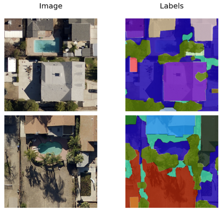
Load model architecture
arcgis.learn provides the MaXDeepLab model for panoptic segmentation task.
model = MaXDeepLab(data)Find an optimal learning rate
Learning rate is one of the most important hyperparameters in model training. The ArcGIS API for Python provides a learning rate finder that automatically chooses the optimal learning rate for you.
lr = model.lr_find()
lr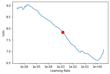
0.001445439770745928
Fit the model
Next, we will train the model for a few epochs with the learning rate found above. We have trained the model using a large dataset for 20 epochs. If the loss continues to decrease, the model can be trained further until you start seeing overfitting.
model.fit(20, lr=lr)| epoch | train_loss | valid_loss | time |
|---|---|---|---|
| 0 | 3.013765 | 2.962664 | 51:13 |
| 1 | 2.951099 | 2.877245 | 51:03 |
| 2 | 2.817451 | 2.777940 | 51:42 |
| 3 | 2.777210 | 2.683472 | 51:51 |
| 4 | 2.687376 | 2.612125 | 51:58 |
| 5 | 2.704202 | 2.614944 | 52:02 |
| 6 | 2.564810 | 2.567012 | 52:03 |
| 7 | 2.468962 | 2.545167 | 51:56 |
| 8 | 2.451628 | 2.680915 | 52:14 |
| 9 | 2.397162 | 2.388501 | 52:05 |
| 10 | 2.397524 | 2.368094 | 52:15 |
| 11 | 2.375640 | 2.498320 | 52:06 |
| 12 | 2.300516 | 3.199307 | 52:16 |
| 13 | 2.263059 | 2.327716 | 52:20 |
| 14 | 2.284510 | 2.408677 | 52:10 |
| 15 | 2.257510 | 2.912793 | 52:09 |
| 16 | 2.219707 | 2.212486 | 52:03 |
| 17 | 2.141654 | 2.257819 | 52:08 |
| 18 | 2.161702 | 2.928984 | 52:35 |
| 19 | 2.161809 | 2.332537 | 52:24 |
We can see in the following plot that although the training loss was contantly reducing gradually, the validation loss became erratic after 12th epoch. The smallest validation loss was recorded for the 17th epoch.
MaXDeepLab has a compound loss function - a combination of multiple metrics. It has been observed that longer training with a relatively flat validation loss curve can also improve results. A diverging training and validation loss curve will still reflect overfitting.
model.plot_losses()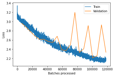
Visualize results in validation set
It is a good practice to see the results of the model viz-a-viz ground truth. The code below picks random samples and shows us ground truth and model predictions, side by side. This enables us to preview the results of the model we trained.
model.show_results(alpha=0.8)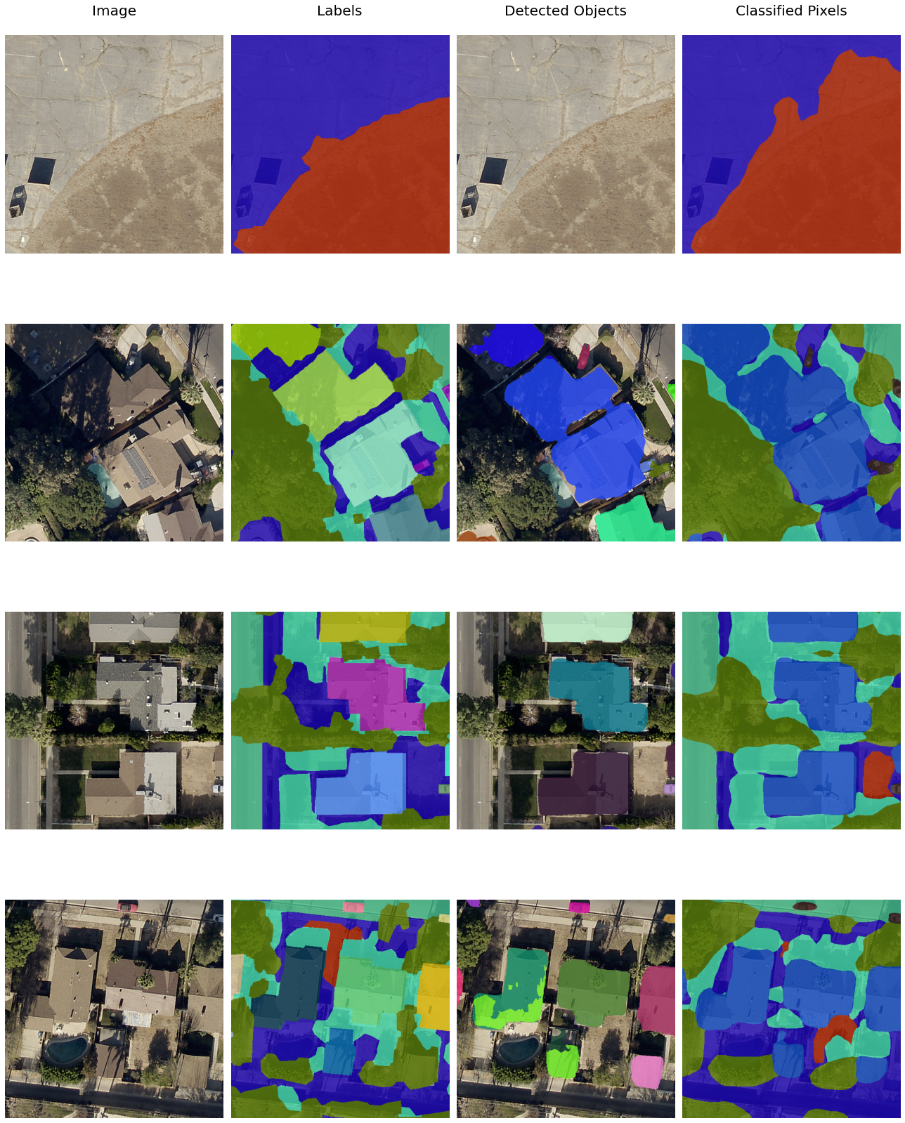
Accuracy assessment
MaXDeepLab provides the panoptic_quality() method that computes the panoptic quality, a combination of recognition and segmentation quality, of the model on the validation set.
model.panoptic_quality()
Save the model
We will save the trained model as a 'Deep Learning Package' ('.dlpk' format). The Deep Learning package is the standard format used to deploy deep learning models on the ArcGIS platform.
We will use the save() method to save the trained model. By default, it will be saved to the 'models' sub-folder within our training data folder.
model.save("la_panoptic_512px_ep21_lr001", publish=True)Deploy the model
We can now use the saved model to detect buildings and cars and classify the LULC. Here, we have provided a very high resolution sample raster for LA County for inferencing. The spatial resolution of the imagery is 0.32 ft and contains 3 bands: Red, Green, and Blue.
sample_inference_raster = gis_ent.content.get('0c8288d76d1c4301ab8b5efbad358f39')
sample_inference_rasterWe have provided a trained model to use for inferencing.
trained_model = gis.content.get('4ef21be1d9fb4ced9eacb306558e8edd')
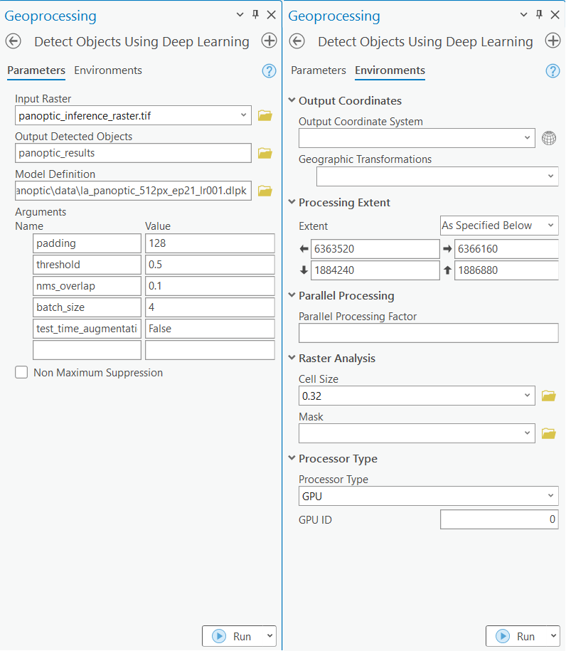
trained_modelIn this step, we will use the Detect Objects Using Deep Learning tool available in both ArcGIS Pro and ArcGIS Enterprise to generate a feature layer with detected buildings and cars and a classified raster with the LULC.
Results
The model was run on the sample inference raster and the results can be viewed here.
fc = gis_ent.content.get('93218b40ca6e471db4456a610d0070d5')
fcic = gis.content.get('ca935d3e3e614e2392485e07ab56b97f')
icVisualize results using map widgets
Two map widgets are created showing the inference raster and the results.
map1 = gis_ent.map()
map1.content.add(inference_raster)
map2 = gis.map()
map2.content.add(fc)
map2.content.add(ic)
The maps are synchronized with each other using MapView.sync_navigation functionality. It helps in comparing the inference raster with the results. Detailed description about advanced map widget options can be referred here.
map2.sync_navigation(map1)from ipywidgets import HBox, VBox, Label, LayoutSet the layout of the map widgets using Hbox and Vbox.
hbox_layout = Layout()
hbox_layout.justify_content = 'space-around'

hb1=HBox([Label('Raster'),Label('Results')])
hb1.layout=hbox_layout
VBox([hb1,HBox([map1,map2])])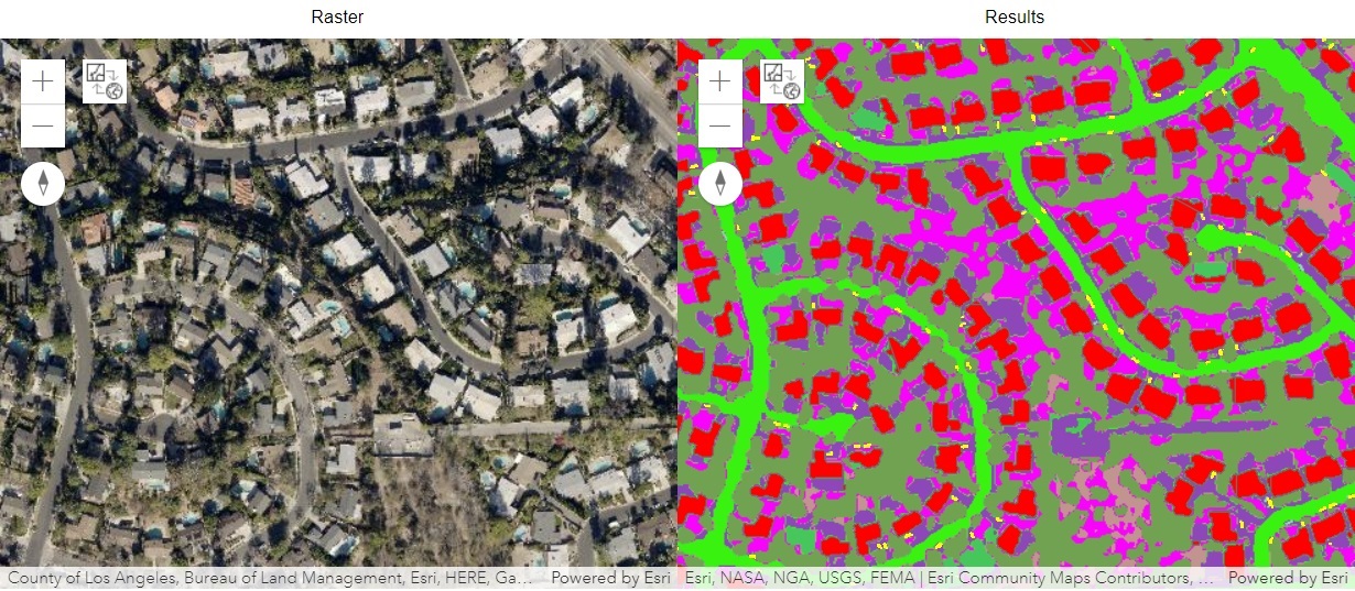
Conclusion
In this notebook we saw how the panoptic segmentation model MaXDeepLab can be used to classify pixels and detect objects at the same time. We learned how to create the data in the Panoptic Segmenation format and use it to train a model using the ArcGIS API for Python. The trained model was then used to generate results for a sample raster and was displayed in the notebook.
