Being able to retrieve, display, analyze, and export the content within an organization Portal are important tasks for any admin. Here we will leverage the ContentManager and UserManager classes of the GIS module, as well as some functionality from the Pandas library, to accomplish those tasks.
Import Libraries
import pandas as pd
from IPython.display import display

import arcgis
from arcgis.gis import GIS
Connect to ArcGIS Online
profile_name = "my_dev_profile"

gis = GIS(profile=profile_name)
gis.users.meQuerying Content
To search for content within our organization, we can access the ContentManager class via gis.content().
Using the advanced_search() method, we can query content belonging to a user by providing the string "owner: < username >". By setting the return_count parameter of advanced_search() to True, we can simply return a single integer representing the number of items which that user owns.
Let's return the number of items that belong to the user currently logged in:
qe = f"owner: {gis.users.me.username}"
my_content_count = gis.content.advanced_search(query=qe,return_count=True)
print(my_content_count, 'items found for current user')
1240 items found for current user
Searching for Content
If we leave the return_count parameter as its default value False, then we will receive a response dictionary containing metadata about the query as well as a list of returned items in the results field.
By setting the max_items parameter, we can limit the number of items that are returned in the results field.
max_items = 3
user_content = gis.content.advanced_search(query=qe, max_items=max_items)
user_content
{'query': 'owner: api_data_owner',
'total': 1240,
'start': 1,
'num': 3,
'nextStart': 4,
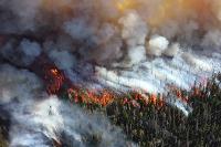
'results': [<Item title:" Exposing patterns in land fires around the globe " type:StoryMap owner:api_data_owner>,
<Item title:" Exposing patterns in land fires around the globe " type:StoryMap owner:api_data_owner>,
<Item title:" Exposing patterns in land fires around the globe " type:StoryMap owner:api_data_owner>]}Displaying Content
# Displaying the result items through IPython.display.display()

for item in user_content['results']:
display(item)It is also possible to have these items returned as dictionary objects by setting the as_dict parameter:
# return items as a dictionary with as_dict=True

user_content_as_dict = gis.content.advanced_search(
    query=qe, max_items=max_items,as_dict=True)
user_content_as_dict['results']
[{'id': 'f1b6a842fbea45bca693c2fe6622bf70',
'owner': 'api_data_owner',
'created': 1610462632000,
'isOrgItem': True,
'modified': 1610462693000,
'guid': None,
'name': None,
'title': ' Exposing patterns in land fires around the globe ',
'type': 'StoryMap',
'typeKeywords': ['arcgis-storymaps',
'smdraftresourceid:draft_1599006014540.json',
'smpublisheddate:1599006014535',
'smstatuspublished',
'smversiondraft:20.35.0',
'smversionpublished:20.35.0',
'source-0f5ef7b723cd410f8e4e298d716bcd73',
'StoryMap',
'Web Application'],
'description': "For decades, the NASA satellites Aqua and Terra have been monitoring potential wildfires with their MODIS sensors. In this StoryMap, I delve into the data archives to look at spatial and temporal patterns and trends.<div><br /></div><div>The\xa0<a href='https://storymaps.arcgis.com/stories/5985c0af444c4fbbb53b92a1bf880503' rel='nofollow ugc' target='_blank'>original StoryMap</a>\xa0has been translated into German, courtesy of\xa0<a href='https://www.esri.de/de-de/home' rel='nofollow ugc' target='_blank'>Esri Deutschland</a>.\xa0</div>",
'tags': ['wildfire',
'fire',
'MODIS',
'satellite',
'ArcGIS Pro',
'spatial analysis'],
'snippet': 'This story map analyzes global patterns in wildfires using spatial analysis tools in ArcGIS Pro with satellite thermal data. ',
'thumbnail': 'thumbnail/ago_downloaded.jpg',
'documentation': None,
'extent': [],
'categories': [],
'spatialReference': None,
'accessInformation': 'Esri',
'licenseInfo': 'No restrictions on use or redistribution.\xa0',
'culture': 'en-us',
'properties': None,
'advancedSettings': None,
'url': 'https://storymaps.arcgis.com/stories/f1b6a842fbea45bca693c2fe6622bf70',
'proxyFilter': None,
'access': 'private',
'size': -1,
'subInfo': 0,
'appCategories': [],
'industries': [],
'languages': [],
'largeThumbnail': None,
'banner': None,
'screenshots': [],
'listed': False,
'ownerFolder': None,
'protected': False,
'numComments': 0,
'numRatings': 0,
'avgRating': 0,
'numViews': 1,
'scoreCompleteness': 96,
'groupDesignations': None,
'contentOrigin': 'self'},
{'id': 'fb2cdb23cece4c49a28e928d70511aa7',
'owner': 'api_data_owner',
'created': 1610515804000,
'isOrgItem': True,
'modified': 1610515854000,
'guid': None,
'name': None,
'title': ' Exposing patterns in land fires around the globe ',
'type': 'StoryMap',
'typeKeywords': ['arcgis-storymaps',
'smdraftresourceid:draft_1599006014540.json',
'smpublisheddate:1599006014535',
'smstatuspublished',
'smversiondraft:20.35.0',
'smversionpublished:20.35.0',
'source-0f5ef7b723cd410f8e4e298d716bcd73',
'StoryMap',
'Web Application'],
'description': " For decades, the NASA satellites Aqua and Terra have been monitoring potential wildfires with their MODIS sensors . In this StoryMap, I delve into the data archives to look at spatial and temporal patterns and trends. <div><br /></div><div> The <a href='https://storymaps.arcgis.com/stories/5985c0af444c4fbbb53b92a1bf880503' rel='nofollow ugc' target='_blank'> original StoryMap </a> has been translated into German, courtesy of <a href='https://www.esri.de/de-de/home' rel='nofollow ugc' target='_blank'> Esri Germany </a> . </div>",
'tags': ['wildfire',
'fire',
'MODIS',
'satellite',
'ArcGIS Pro',
'spatial analysis'],
'snippet': ' This story map analyses global patterns in wildfires using spatial analysis tools in ArcGIS Pro with satellite thermal data . ',
'thumbnail': 'thumbnail/ago_downloaded.jpg',
'documentation': None,
'extent': [],
'categories': [],
'spatialReference': None,
'accessInformation': 'Esri',
'licenseInfo': 'No restrictions on use or redistribution.\xa0',
'culture': 'en-us',
'properties': None,
'advancedSettings': None,
'url': 'https://storymaps.arcgis.com/stories/fb2cdb23cece4c49a28e928d70511aa7',
'proxyFilter': None,
'access': 'private',
'size': -1,
'subInfo': 0,
'appCategories': [],
'industries': [],
'languages': [],
'largeThumbnail': None,
'banner': None,
'screenshots': [],
'listed': False,
'ownerFolder': None,
'protected': False,
'numComments': 0,
'numRatings': 0,
'avgRating': 0,
'numViews': 1,
'scoreCompleteness': 98,
'groupDesignations': None,
'contentOrigin': 'self'},
{'id': '7bfce9c3f0734d5896584b21d8fc2ba9',
'owner': 'api_data_owner',
'created': 1613391382000,
'isOrgItem': True,
'modified': 1613391500000,
'guid': None,
'name': None,
'title': ' Exposing patterns in land fires around the globe ',
'type': 'StoryMap',
'typeKeywords': ['arcgis-storymaps',
'smdraftresourceid:draft_1599006014540.json',
'smpublisheddate:1599006014535',
'smstatuspublished',
'smversiondraft:20.35.0',
'smversionpublished:20.35.0',
'source-0f5ef7b723cd410f8e4e298d716bcd73',
'StoryMap',
'Web Application'],
'description': " For decades, the NASA satellites Aqua and Terra have been monitoring potential wildfires with their MODIS sensors . In this StoryMap, I delve into the data archives to look at spatial and temporal patterns and trends. <div><br /></div><div> The <a href='https://storymaps.arcgis.com/stories/5985c0af444c4fbbb53b92a1bf880503' rel='nofollow ugc' target='_blank'> original StoryMap </a> has been translated into German, courtesy of <a href='https://www.esri.de/de-de/home' rel='nofollow ugc' target='_blank'> Esri Germany </a> . </div>",
'tags': ['wildfire',
'fire',
'MODIS',
'satellite',
'ArcGIS Pro',
'spatial analysis'],
'snippet': ' This story map analyses global patterns in wildfires using spatial analysis tools in ArcGIS Pro with satellite thermal data . ',
'thumbnail': 'thumbnail/ago_downloaded.jpg',
'documentation': None,
'extent': [],
'categories': [],
'spatialReference': None,
'accessInformation': 'Esri',
'licenseInfo': 'No restrictions on use or redistribution.\xa0',
'culture': 'en-us',
'properties': None,
'advancedSettings': None,
'url': 'https://storymaps.arcgis.com/stories/7bfce9c3f0734d5896584b21d8fc2ba9',
'proxyFilter': None,
'access': 'private',
'size': -1,
'subInfo': 0,
'appCategories': [],
'industries': [],
'languages': [],
'largeThumbnail': None,
'banner': None,
'screenshots': [],
'listed': False,
'ownerFolder': None,
'protected': False,
'numComments': 0,
'numRatings': 0,
'avgRating': 0,
'numViews': 0,
'scoreCompleteness': 98,
'groupDesignations': None,
'contentOrigin': 'self'}]Sorting Content
The sort_field and sort_order parameters of the advanced_search() method can be used to sort the returned content server side.
Possible values for sort_order are "asc" for ascending or increasing order and "desc" for descending or decreasing order. Default values for the sort_field and sort_order parameters are "title" and "asc", respectively.
In this next example we'll search for the last 3 items that the current user modified by setting sort_field="modified" and sort_order="desc":
content_last_modified = gis.content.advanced_search(
    query=qe, max_items=max_items, sort_field="modified", sort_order="desc")

for item in content_last_modified['results']:
display(item)Here we return the first 3 items that the user created by setting sort_field="created" and sort_order="asc":
content_first_created = gis.content.advanced_search(query=qe, max_items=max_items, sort_field="created", sort_order="asc")

for item in content_first_created['results']:
display(item)Querying Organization Content
Searching for Organization Members
We can search for a list of the members within the organization by using the UserManager class within the GIS module. Here we access the UserManager by calling gis.users, and use the search() method to return a list of organization members. The search() method will return all users in the organization if no parameters are provided:
# View UserManager object
gis.users
<UserManager @ https://geosaurus.maps.arcgis.com>
org_users = gis.users.search()
print(f'{len(org_users)} users found')
org_users[:3]
42 users found
[<User username:achapkowski_geosaurus>,
 <User username:amani_geosaurus>,
 <User username:andrew57>]
# Display a misc member
org_member = org_users[1]
org_memberGetting Member Content
Similarly to above, we can set return_count=True and see how many items this user has:
# See the number of member items
qe = "owner: " + org_member.username
member_content_count = gis.content.advanced_search(
    query=qe, max_items=-1, return_count=True)
print(f"Org member has {member_content_count} items")
Org member has 24 items
# Return <max_items> items from member
max_items = 3

member_content = gis.content.advanced_search(query=qe, max_items=max_items)
member_content['results']
[<Item title:"Demo Initiative1" type:Hub Site Application owner:amani_geosaurus>, <Item title:"Demo Initiative1" type:Hub Initiative owner:amani_geosaurus>, <Item title:"geotaggedphotos1" type:Feature Layer Collection owner:amani_geosaurus>]
Compiling Organization Content
If we return all items for each user in the organization, we can compile those items into a single list representing all of the organizations content.
We can remove the item limit for each query by setting max_items=-1 in the advanced_search() function:
# return content for each user in org, compile into a single list

org_content = []

for user in org_users:
    qe = f"owner: {user.username}"
    user_content = gis.content.advanced_search(query=qe, max_items=-1)['results']
    org_content += user_content

print(f"{len(org_content)} items found in org")
1848 items found in org
Analyzing Organization Content with Pandas
Let's put our compiled list into a pandas DataFrame to easily view and filter our data
# Create DataFrame

content_df = pd.DataFrame(org_content)
content_df.head()| id | owner | created | isOrgItem | modified | guid | name | title | type | typeKeywords | ... | size | ownerFolder | commentsEnabled | itemControl | layers | tables | appProxies | protected | contentStatus | sourceUrl | |
|---|---|---|---|---|---|---|---|---|---|---|---|---|---|---|---|---|---|---|---|---|---|
| 0 | 8ec563a6886f474c8d991e7748ab4c03 | amani_geosaurus | 1558567624000 | True | 1558567631000 | None | None | Demo Initiative1 | Hub Site Application | [Hub, hubSite, hubSolution, JavaScript, Map, M... | ... | 95654.0 | None | True | update | NaN | NaN | NaN | NaN | NaN | NaN |
| 1 | d1d2876870ab422488e425db4c400361 | amani_geosaurus | 1558567621000 | True | 1558567632000 | None | None | Demo Initiative1 | Hub Initiative | [Hub, hubInitiative, OpenData] | ... | NaN | NaN | NaN | NaN | NaN | NaN | NaN | NaN | NaN | NaN |
| 2 | 72567bd147fd478da9563bc56b434870 | amani_geosaurus | 1634162116000 | True | 1634162156000 | None | geotaggedphotos1 | geotaggedphotos1 | Feature Service | [ArcGIS Server, Data, Feature Access, Feature ... | ... | NaN | NaN | NaN | NaN | NaN | NaN | NaN | NaN | NaN | NaN |
| 3 | 6fd3252f1ad044869dd4f949ea4b20cc | amani_geosaurus | 1555049137000 | True | 1555049257000 | None | None | hu_indy_18p | Feature Service | [ArcGIS Server, Data, Feature Access, Feature ... | ... | NaN | NaN | NaN | NaN | NaN | NaN | NaN | NaN | NaN | NaN |
| 4 | 1d3614ec5cc24382878533f8454c24a3 | amani_geosaurus | 1630112960000 | True | 1630112990000 | None | 1d3614ec5cc24382878533f8454c24a3.ipynb | intro to notebooks | Notebook | [Notebook, Python] | ... | NaN | NaN | NaN | NaN | NaN | NaN | NaN | NaN | NaN | NaN |
5 rows × 51 columns
We can use the pandas function value_counts() to see how many occurrences there are of each value for a particular column. Here we return the top 10 most frequently occurring item types and the number of instances they have:
# use value_counts() to see how many items you have with a particular key:value pair
content_df.type.value_counts().head(10)
Feature Service 435 Feature Collection 429 Notebook 342 Shapefile 129 StoryMap 98 Service Definition 76 Image Collection 65 File Geodatabase 43 Deep Learning Package 43 Web Map 33 Name: type, dtype: int64
Another value_counts() example where we see the distribution of access levels for each of the items in the organization:
content_df.access.value_counts()private 815 org 518 public 513 shared 2 Name: access, dtype: int64
Using the value_counts() function in conjunction with the groupby() operation allows for an additional level of analysis. Here we see the breakdown of item types that each user has created:
content_df.groupby('owner').type.value_counts().head(10)owner type
ArcGISPyAPIBot Notebook 31
Feature Service 4
CSV 1
StoryMap 1
Web Map 1
DavidJVitale Feature Service 1
Web Map 1
MMajumdar_geosaurus Hub Site Application 1
amani_geosaurus Feature Service 6
Notebook 4
Name: type, dtype: int64# Viewing the number item types per access level within the org
content_df.groupby('type').access.value_counts().head(10)type access
API Key private 1
Application public 1
CSV public 9
private 8
CSV Collection private 2
public 1
Code Attachment public 2
Code Sample public 6
Dashboard public 5
org 2
Name: access, dtype: int64Filtering the Dataset
We can choose which columns we'd like to view, and the order we'd like to view them in, by providing the DataFrame with a list of strings matching column names:
view_columns = ['id','title','owner','type','access']
content_df[view_columns].head()| id | title | owner | type | access | |
|---|---|---|---|---|---|
| 0 | 8ec563a6886f474c8d991e7748ab4c03 | Demo Initiative1 | amani_geosaurus | Hub Site Application | org |
| 1 | d1d2876870ab422488e425db4c400361 | Demo Initiative1 | amani_geosaurus | Hub Initiative | org |
| 2 | 72567bd147fd478da9563bc56b434870 | geotaggedphotos1 | amani_geosaurus | Feature Service | org |
| 3 | 6fd3252f1ad044869dd4f949ea4b20cc | hu_indy_18p | amani_geosaurus | Feature Service | public |
| 4 | 1d3614ec5cc24382878533f8454c24a3 | intro to notebooks | amani_geosaurus | Notebook | public |
Creating and applying Boolean masks is a very efficient way to the filter the rows of a DataFrame. By using standard operators such as <, >, == and != on pandas Series objects (e.g. the columns of our DataFrame), we can create a new Series of True and False values, called a mask. When this mask is applied to the original DataFrame, a new DataFrame will be returned with only the rows corresponding to where the mask had a True value.
Let's create a mask to represent all items with public level access:
filter_value = 'public'
filter_column = 'access'
row_filter = content_df[filter_column]==filter_value
row_filter.head()
0 False 1 False 2 False 3 True 4 True Name: access, dtype: bool
Applying this mask to our DataFrame, we return all fields for objects which have access=='public':
print(len(content_df[row_filter]), 'objects in filtered DataFrame')
content_df[row_filter].head()
513 objects in filtered DataFrame
| id | owner | created | isOrgItem | modified | guid | name | title | type | typeKeywords | ... | size | ownerFolder | commentsEnabled | itemControl | layers | tables | appProxies | protected | contentStatus | sourceUrl | |
|---|---|---|---|---|---|---|---|---|---|---|---|---|---|---|---|---|---|---|---|---|---|
| 3 | 6fd3252f1ad044869dd4f949ea4b20cc | amani_geosaurus | 1555049137000 | True | 1555049257000 | None | None | hu_indy_18p | Feature Service | [ArcGIS Server, Data, Feature Access, Feature ... | ... | NaN | NaN | NaN | NaN | NaN | NaN | NaN | NaN | NaN | NaN |
| 4 | 1d3614ec5cc24382878533f8454c24a3 | amani_geosaurus | 1630112960000 | True | 1630112990000 | None | 1d3614ec5cc24382878533f8454c24a3.ipynb | intro to notebooks | Notebook | [Notebook, Python] | ... | NaN | NaN | NaN | NaN | NaN | NaN | NaN | NaN | NaN | NaN |
| 5 | 67ec03dba0d44bb1924cd8b3aebf2db4 | amani_geosaurus | 1613548980000 | True | 1613548981000 | None | KMZ_ContentType_Region_UnitedNations-3.zip | KMZ_ContentType_Region_UnitedNations-3 | KML Collection | [KML Collection] | ... | NaN | NaN | NaN | NaN | NaN | NaN | NaN | NaN | NaN | NaN |
| 6 | 8df836df4d544067b715c296608beea4 | amani_geosaurus | 1591834702000 | True | 1591860089000 | None | None | Lambda requests on a map | Web Map | [ArcGIS Online, Explorer Web Map, Map, Online ... | ... | NaN | NaN | NaN | NaN | NaN | NaN | NaN | NaN | NaN | NaN |
| 7 | 8443e3c2473549f0b464a6a3f295acf9 | amani_geosaurus | 1591655624000 | True | 1591655626000 | None | None | lambda-credit-counter | Application | [Application, Registered App] | ... | NaN | NaN | NaN | NaN | NaN | NaN | NaN | NaN | NaN | NaN |
5 rows × 51 columns
We can apply both the column filter and Boolean mask at the same time to reduce the amount of information displayed:
content_df[row_filter][view_columns].head()| id | title | owner | type | access | |
|---|---|---|---|---|---|
| 3 | 6fd3252f1ad044869dd4f949ea4b20cc | hu_indy_18p | amani_geosaurus | Feature Service | public |
| 4 | 1d3614ec5cc24382878533f8454c24a3 | intro to notebooks | amani_geosaurus | Notebook | public |
| 5 | 67ec03dba0d44bb1924cd8b3aebf2db4 | KMZ_ContentType_Region_UnitedNations-3 | amani_geosaurus | KML Collection | public |
| 6 | 8df836df4d544067b715c296608beea4 | Lambda requests on a map | amani_geosaurus | Web Map | public |
| 7 | 8443e3c2473549f0b464a6a3f295acf9 | lambda-credit-counter | amani_geosaurus | Application | public |
Another example where we create a Boolean mask for all objects of type "Web Map":
filter_value = 'Web Map'
filter_column = 'type'
row_filter = content_df[filter_column]==filter_value
content_df[row_filter][view_columns]| id | title | owner | type | access | |
|---|---|---|---|---|---|
| 6 | 8df836df4d544067b715c296608beea4 | Lambda requests on a map | amani_geosaurus | Web Map | public |
| 23 | 5776d859b5a84b1b96d5c5bbfcc0d3d3 | WebMap for Landfall Spotlight Article | amani_geosaurus | Web Map | public |
| 36 | 81ef30218b3f41e89019160faa4de099 | Headless WebMap about Parks | andrew57 | Web Map | public |
| 38 | 54fd67f260fe413da84ed4f2d9e1dac2 | National Levee Database Map | andrew57 | Web Map | public |
| 44 | a478d4172870462dae95d0b26561e3ac | SarahAWebMapSample | andrew57 | Web Map | org |
| 46 | ac02f94f0b8d42e59c74fdf9fb249a06 | VectorTileFromOtherSiteLayerandBasemap | andrew57 | Web Map | public |
| 96 | 127a87ebeede4e6c919d43b600763a3b | Addresses Geocoded | api_data_owner | Web Map | private |
| 291 | 7d76c6397380497f9879df74f80f0214 | Brick Kilns around Jaipur 2019 | api_data_owner | Web Map | public |
| 292 | e91b9226ef224e7da4f32cb034c8b94d | Brick Klinks around Delhi 2014 | api_data_owner | Web Map | public |
| 293 | 711b1725f6334aeca2151734b37d3c50 | Brick Klinks around Delhi 2019 | api_data_owner | Web Map | public |
| 406 | 6527ca7eea2a4cad826e11f298d09500 | Coastline_India | api_data_owner | Web Map | public |
| 407 | a3e8eda445c34e95bdef7aa75bdd8a77 | Coastline_India_l8 | api_data_owner | Web Map | public |
| 483 | 7d4f5249de15493a9916c03e509b831c | slums_2004 | api_data_owner | Web Map | public |
| 484 | f3f7d8c728e74230baeed747a5322ba5 | slums_2014 | api_data_owner | Web Map | public |
| 542 | 2fecd25df8624a41b15dfc97ed4c8f98 | Superresolution Inferenced Map | api_data_owner | Web Map | public |
| 557 | 2051a50d9370428297dc08a87db4a43f | oma-test-map | api_data_owner | Web Map | org |
| 558 | 7cb38a3325564607a81c0da5733bfbfc | oma-test-map-updates | api_data_owner | Web Map | private |
| 559 | 966cba4a3bfe487692b305d923fe2777 | oma-test-map-updates-052220 | api_data_owner | Web Map | private |
| 573 | 6b43fb3f165245e3b72eba2ff2357d98 | Parcel_extraction_results_e02 | api_data_owner | Web Map | private |
| 823 | 2303b34ac97b4689bd5ff851d5982a96 | USA_coastline | api_data_owner | Web Map | public |
| 870 | 66db719c5a7844a0b681876f7cd4c269 | wm-test-n-layers | api_data_owner | Web Map | org |
| 871 | d0772d26a75141f9ac11998c16b06eed | wm-test-n-layers-dgray | api_data_owner | Web Map | org |
| 923 | 7fe016b30663401baf415f4dd1078d36 | Extracted land parcels | api_data_owner | Web Map | public |
| 1311 | 6d8e89f6fb0a4c8a8bb5e059846425d9 | Giraffes | ArcGISPyAPIBot | Web Map | org |
| 1338 | b270d508a6354c6c84510e83f94ebf19 | API_downloads_across_globe | arcgis_python | Web Map | org |
| 1376 | ebc72a274dff4315b703e5de0a894831 | Location Allocation example of Pizza Stores in... | arcgis_python | Web Map | public |
| 1378 | 27a956e9da094da98ebba3312a456078 | Map_View_Google Drive Image | arcgis_python | Web Map | public |
| 1380 | e66622a75ac14fffaf2e8223025479a0 | Mobiliario Madrid | arcgis_python | Web Map | public |
| 1802 | c0da3fa83cd34379b49c56a33247910b | wMap5_withCharts | arcgis_python | Web Map | public |
| 1803 | 393e05923b7c4d289d305273b30a1ea3 | testing | DavidJVitale | Web Map | public |
| 1808 | 3c9ab685601748b9b55f06c6a529d070 | Chicago Libraries 2012 | jyaist_geosaurus | Web Map | org |
| 1811 | 4aeed784e57043e49895293e576f732a | Guinea Power Plants | jyaist_geosaurus | Web Map | shared |
| 1835 | 0c4170b6934245269ffc3f41acbb4a87 | LeafPickupMap | naubry_geosaurus | Web Map | org |
Boolean masks can also be combined to represent multiple filters. Here we combine the Web Map and Public masks to return all items in our organization which are public web maps:
# Combining masks
web_map_filter = content_df.type=='Web Map'
public_filter = content_df.access=='public'
combined_mask = web_map_filter & public_filter

content_df[combined_mask][view_columns]| id | title | owner | type | access | |
|---|---|---|---|---|---|
| 6 | 8df836df4d544067b715c296608beea4 | Lambda requests on a map | amani_geosaurus | Web Map | public |
| 23 | 5776d859b5a84b1b96d5c5bbfcc0d3d3 | WebMap for Landfall Spotlight Article | amani_geosaurus | Web Map | public |
| 36 | 81ef30218b3f41e89019160faa4de099 | Headless WebMap about Parks | andrew57 | Web Map | public |
| 38 | 54fd67f260fe413da84ed4f2d9e1dac2 | National Levee Database Map | andrew57 | Web Map | public |
| 46 | ac02f94f0b8d42e59c74fdf9fb249a06 | VectorTileFromOtherSiteLayerandBasemap | andrew57 | Web Map | public |
| 291 | 7d76c6397380497f9879df74f80f0214 | Brick Kilns around Jaipur 2019 | api_data_owner | Web Map | public |
| 292 | e91b9226ef224e7da4f32cb034c8b94d | Brick Klinks around Delhi 2014 | api_data_owner | Web Map | public |
| 293 | 711b1725f6334aeca2151734b37d3c50 | Brick Klinks around Delhi 2019 | api_data_owner | Web Map | public |
| 406 | 6527ca7eea2a4cad826e11f298d09500 | Coastline_India | api_data_owner | Web Map | public |
| 407 | a3e8eda445c34e95bdef7aa75bdd8a77 | Coastline_India_l8 | api_data_owner | Web Map | public |
| 483 | 7d4f5249de15493a9916c03e509b831c | slums_2004 | api_data_owner | Web Map | public |
| 484 | f3f7d8c728e74230baeed747a5322ba5 | slums_2014 | api_data_owner | Web Map | public |
| 542 | 2fecd25df8624a41b15dfc97ed4c8f98 | Superresolution Inferenced Map | api_data_owner | Web Map | public |
| 823 | 2303b34ac97b4689bd5ff851d5982a96 | USA_coastline | api_data_owner | Web Map | public |
| 923 | 7fe016b30663401baf415f4dd1078d36 | Extracted land parcels | api_data_owner | Web Map | public |
| 1376 | ebc72a274dff4315b703e5de0a894831 | Location Allocation example of Pizza Stores in... | arcgis_python | Web Map | public |
| 1378 | 27a956e9da094da98ebba3312a456078 | Map_View_Google Drive Image | arcgis_python | Web Map | public |
| 1380 | e66622a75ac14fffaf2e8223025479a0 | Mobiliario Madrid | arcgis_python | Web Map | public |
| 1802 | c0da3fa83cd34379b49c56a33247910b | wMap5_withCharts | arcgis_python | Web Map | public |
| 1803 | 393e05923b7c4d289d305273b30a1ea3 | testing | DavidJVitale | Web Map | public |
The apply() method can also be used to generate masks that can't be created using the standard comparison operators. As long as the function called within the apply method has a Boolean output, then the result can be used as a mask to filter rows. Here we use a lambda function to return all items which have a type that ends with the word "Service".
# Creating masks with .apply and lambda functions

service_filter = content_df.type.apply(lambda x: x.endswith('Service'))
content_df[service_filter][view_columns]| id | title | owner | type | access | |
|---|---|---|---|---|---|
| 2 | 72567bd147fd478da9563bc56b434870 | geotaggedphotos1 | amani_geosaurus | Feature Service | org |
| 3 | 6fd3252f1ad044869dd4f949ea4b20cc | hu_indy_18p | amani_geosaurus | Feature Service | public |
| 9 | d77abcdc3f04488f84ad22bc7afdfcad | Landfall density 2 | amani_geosaurus | Map Service | public |
| 11 | ffef49c345154bc5b24c8e2e39587ec4 | Landfall Spotlight Article_WFL1 | amani_geosaurus | Feature Service | public |
| 19 | e0959e7018914be0931a9f15efb56c94 | request_locations | amani_geosaurus | Feature Service | public |
| ... | ... | ... | ... | ... | ... |
| 1830 | f129290c5da14d7884b26951eddd6b29 | KingCo_PropertyInfo | maggarwal_geosaurus | Feature Service | public |
| 1832 | af59408fd19a4a1c99e14ff09967e394 | Uganda_Boundary | maggarwal_geosaurus | Feature Service | public |
| 1834 | 42e944d92e1346f5a4229aa76841e5c2 | Leaf_Pickup_Routes | naubry_geosaurus | Feature Service | org |
| 1837 | 1cc19cce694e4caf95ce4471befd55b7 | Vexcel_Houston_Nadir | rohitgeo | Image Service | public |
| 1846 | b120ffa7170f4be0b5aaad8a284c6be5 | Trailheads | yjiang_geosaurus | Feature Service | public |
451 rows × 5 columns
Accessing Content by ID
Once we've identified an item of interest in our DataFrame, we can return the content of that item by providing its ID to the ContentManager get() method. If we know the index of the object in the DataFrame (i.e. the leftmost value), then we can access that row's information using the loc() method. From there we can get the id of the item and provide it to the get method.
# Return the index of the last item in the previous output
# In this example the index column is labelled 'name'

target_index = content_df[service_filter].iloc[-1].name
print("Target index:", target_index)
Target index: 1846
# Accessing items with content.get()
target_data = content_df.loc[target_index]
print(target_data.id)
target_content = gis.content.get(target_data.id)
target_content
b120ffa7170f4be0b5aaad8a284c6be5
For more information on using item ids, see this community post.
Exporting Data
Pandas provides a convenient to_csv() method which can be used to generate zipped and unzipped csv outputs. Simply provide your target path with the appropriate file extension and call the method on the DataFrame object you would like to export.
# Exporting data to a csv
target_path = "org_content.csv"
content_df.to_csv(target_path)
# Exporting data to gzipped csv file
target_path_gzip = "org_content.csv.gz"
content_df.to_csv(target_path_gzip)# Exporting data to zipped csv file
target_path_zip = "org_content.csv.zip"
content_df.to_csv(target_path_zip)Pandas also provides additional methods for exporting the data as different file formats (e.g. to_json(), to_pickle(), to_excel()) which behave similarly.


