Introduction
Generally, multispectral imagery is preferred for Landuse Landcover (LULC) classification, due to its high temporal resolution and high spatial coverage. With the advances in remote sensing technologies, hyperspectral images are now also a good option for LULC classification, due to their high spectral resolution. The main difference between multispectral and hyperspectral imagery, is the number of bands and how narrow those bands are. One of the advantages hyperspectral sensors have over multispectral sensors is the ability to differentiate within classes. For instance, due to the high spectral information content that creates a unique spectral curve for each class, hyperspectral sensors can distinguish by tree or crop species.
Multispectral imagery

Hyperspectral imagery

In this notebook, we will use hyperspectral data to train a deep learning model and will see if the model can extract subclasses of two LULC classes: developed areas and forests. Hyperion imagery is used in the current analysis to classify the types of forests and developed areas. The data can be downloaded from USGS earth explorer.
Hyperion data preparation
The Earth Observing-1 (EO-1) satellite was launched November 21, 2000 as a one-year technology demonstration/validation mission. After the initial technology mission was completed, NASA and the USGS agreed to the continuation of the EO-1 program as an Extended Mission. The EO-1 Extended Mission is chartered to collect and distribute Hyperion hyperspectral and Advanced Land Imager (ALI) multispectral products according to customer tasking requests.
Hyperion collects 220 unique spectral channels ranging from 0.357 to 2.576 micrometers with a 10-nm bandwidth. The instrument operates in a pushbroom fashion, with a spatial resolution of 30 meters for all bands. The standard scene width is 7.7 kilometers.
Download hyperion imagery
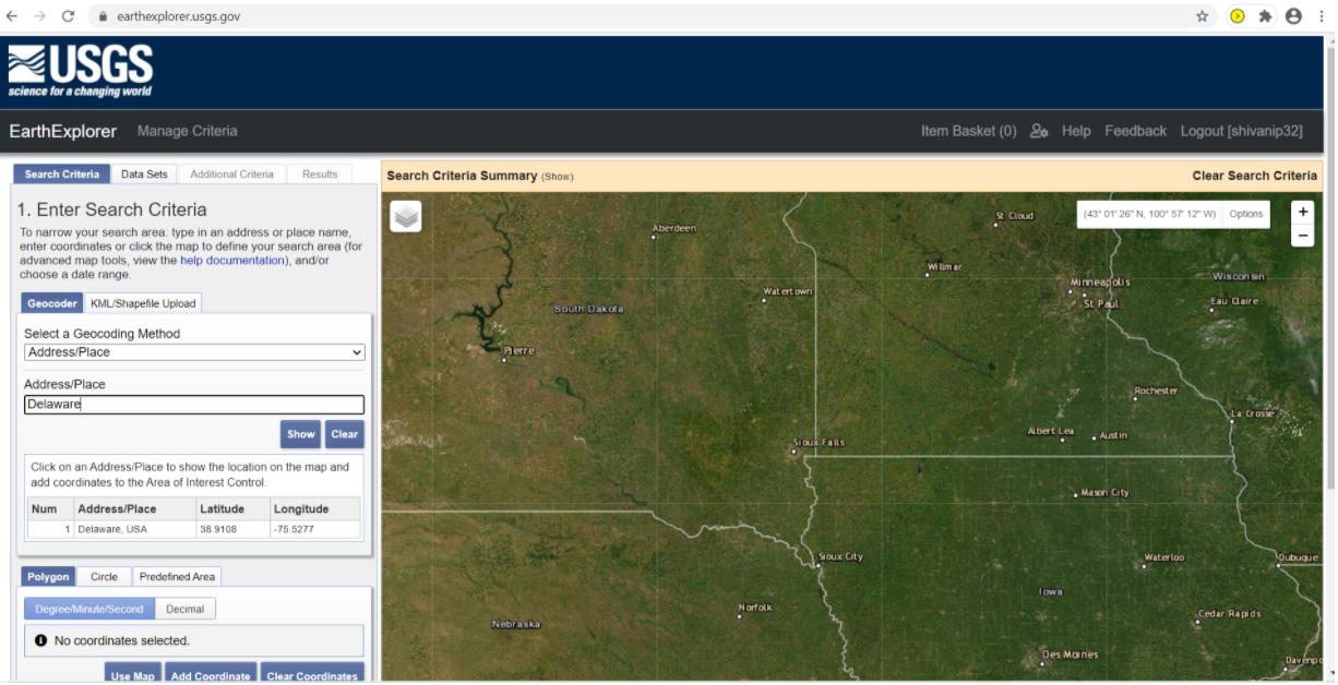
Login to the earth explorer using the USGS credentials. Then, select the Address/Place option in the Geocoding Method dropdown and write the name or address of the area of interest.
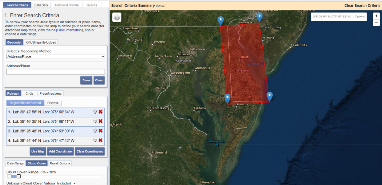
Draw a polygon over the area of interest and change the Cloud Cover Range to 0% - 10%. Click on Results in the bottom left.
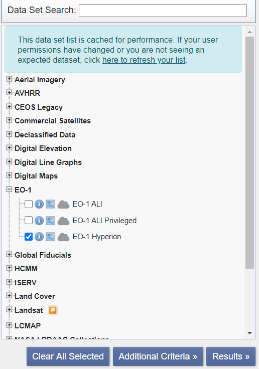
Next, expand EO-1, select EO-1 Hyperion, and click on Results.
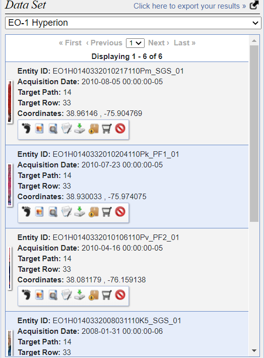
Download the data from the product list.
Pre processing of hyperion imagery
Remove bad bands
Not all bands are useful for analysis. Bad bands are primarily water vapor bands consists inforation about atmosphere, that cause spikes in the reflectance curve. List of bad bands of the Hyperion sensor, L1R product are: 1 to 7 - Not illuminated
58 to 78 - Overlap region
120 to 132 - Water vapor absorption band
165 to 182 - Water vapor absorption band
185 to 187 - Identified by Hyperion bad band list
221 to 224 - Water vapor absorption band
225 to 242 - Not illuminated
Bands with vertical stripping - (8-9, 56-57, 78-82, 97-99, 133-134, 152-153, 188, 213-216, 219-220)
Create composite rasters
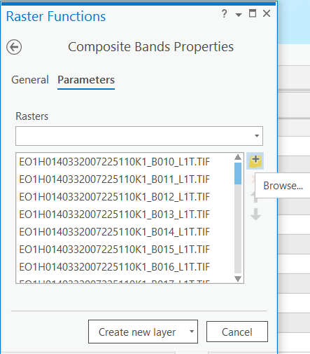
Two sets of composite rasters were created using Composite bands function. The band range of two raster composites are as follows: Two sets of composite rasters were created using the Composite bands function function. The band range of the two raster composites are as follows:
NIR & visible composite - 9 to 55
SWIR composite - 82-96, 100-119, 135-164, 183-184, 189-212, 217-218
Click on Imagery tab -> click on Raster Functions -> Search "Composite Bands" -> Click on browse button and select the bands -> After selecting the bands, click on Create new layer.
Convert DN values to at-sensor radiance
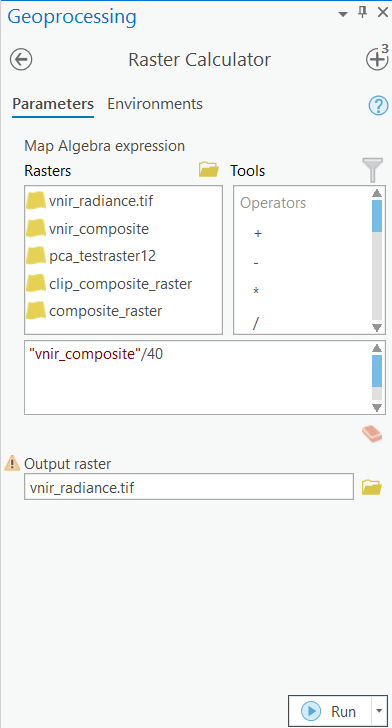
Scale factors will be used to convert the pixel DN value to at-sensor radiance. A scale factor of 40 will be used for the VNIR composite raster and a scale factor of 80 will be used for the SWIR composite. The rasters will be divided by the scale factor using the Raster Calculator tool in ArcGIS Pro.
Create combined composite raster
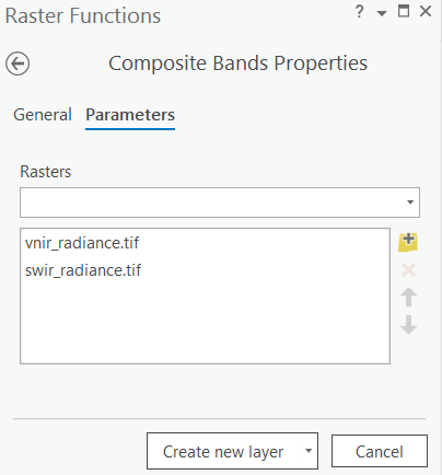
Combine both the VNIR and SWIR radiance composite rasters using the "Composite Band" function.
Eliminate NoData pixels
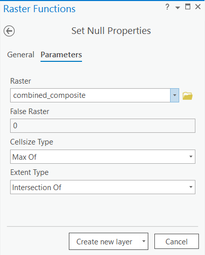
Create null raster
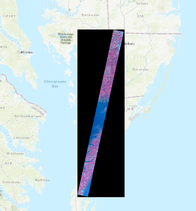
The output raster has a 0 pixel value for NoData that is shown as a black pixel. The NoData pixels can be eliminated using the Set Null tool.
Use the following parameters:
Raster: combined_composite
False raster = 0
Cellsize Type = Max Of
Extent Type = Intersection Of
Clip
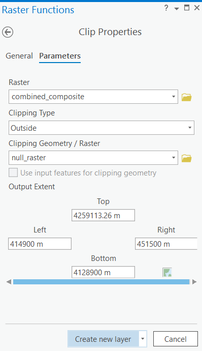
The Clip tool will be used to eliminate instances of NoData from the combined composite raster using the null raster that was created in the previous step.
The input parameters are as follows:
Raster: combined_composite
Clipping Type: Outside
Clipping Geometry/Raster: null_raster
Principal Component Analysis
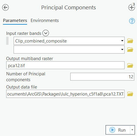
Principle component analysis can be used to determine the comparatively higher information bands of Hyperion's 224 total bands. Principal Components performs Principal Component Analysis (PCA) on a set of raster bands and generates a single multiband raster as its output. The value specified for the number of principal components determines the number of principal component bands in the output multiband raster. The number must not be larger than the total number of raster bands in the input.
The input parameters are as follows:
Input raster bands: Clip_combined_composite
Number of Principal components: 12 (12 Principal component were chosen because they cover more than 98% of the total variance)
The output raster will have 12 bands representing 12 Principal components.
Export training data for deep learning model
from arcgis.gis import GIS
gis = GIS(profile="your_online_profile")
ent_gis = GIS(profile='your_enterprise_profile')
The raster generated from the Hyperion imagery through the Principal Components tool will be used as the input raster for the training data.
pca_raster = ent_gis.content.get('0d86c3f9dedc4566a7cb3d2c18d1ffef')
pca_rasterThe following feature layer will be used as label for training the model.
lulc_polygons = ent_gis.content.get('f69011a01c39494bade9b30708bce064')
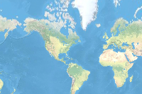
lulc_polygonsm = gis.map('USA')
m.content.add(lulc_polygons)
m.legend.enabled=True
m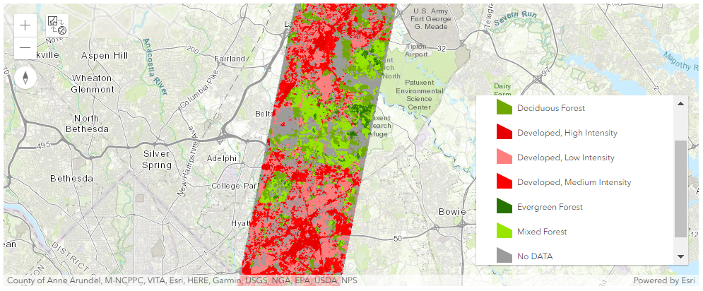
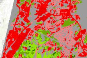
The above layer consists of 7 classes. Developed areas have three sub classes: High, Medium, and Low density areas and Forested areas have 3 types of forests: Evergreen, Mixed, and Deciduous forest. No DATA represents all other LULC classes.
m.zoom_to_layer(lulc_polygons)A feature layer will be used as a input mask polygon while exporting the training data to define the extent of the study area.
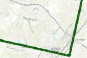
mask_poly = ent_gis.content.get('bfe7bb7ea8454d9384cb8005a5c0f855')
mask_polyThe Export training data for deep learning tool is used to prepare training data for training a deep learning model. The tool is available in both ArcGIS Pro and ArcGIS Enterprise.
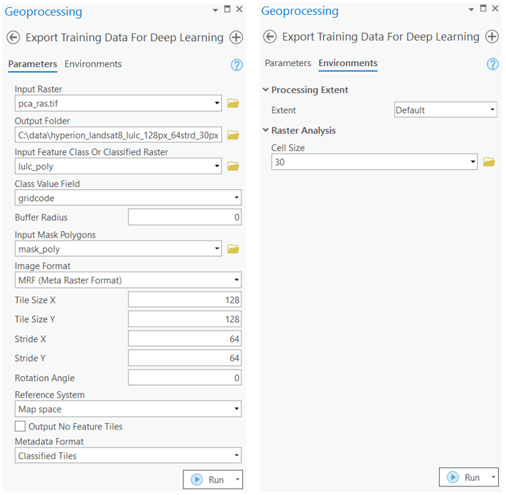
Model training
This step will utilize Jupyter Notebooks, and documentation on how to install and setup the environment is available here.
Necessary Imports
import os
from pathlib import Path

import arcgis
from arcgis.learn import prepare_data, UnetClassifier
Get training data
We have already exported the data, and it can be directly downloaded using the following steps:
training_data = gis.content.get('0a8ff4ce9f734bb5bb72104aea8526af')
training_datafilepath = training_data.download(file_name=training_data.name)import zipfile
with zipfile.ZipFile(filepath, 'r') as zip_ref:
zip_ref.extractall(Path(filepath).parent)data_path = Path(os.path.join(os.path.splitext(filepath)[0]))Visualize training data
The prepare_data function takes a training data path as input and creates a fast.ai databunch with specified transformation, batch size, split percentage, etc.
data = prepare_data(data_path,
                    batch_size=8)
To get a sense of what the training data looks like, use the show_batch() method to randomly pick a few training chips and visualize them. The chips are overlaid with masks representing the building footprints in each image chip.
data.show_batch(alpha=1)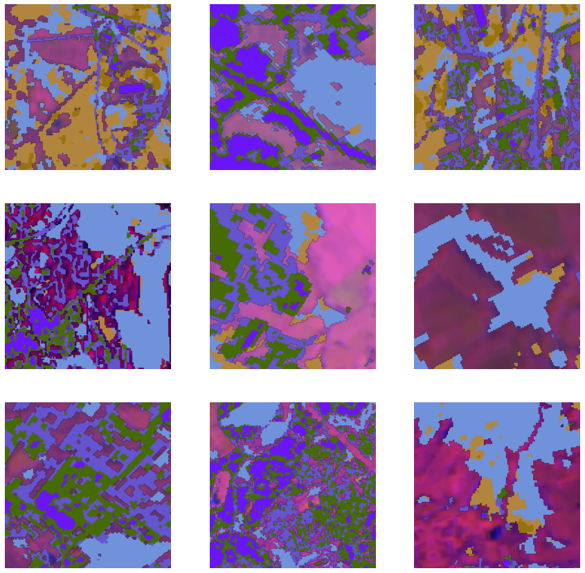
Load model architecture
arcgis.learn provides the UnetClassifier model for per pixel classification that is based on a pretrained convnet, like ResNet, that acts as the 'backbone'. More details about UnetClassifier can be found here.
model = UnetClassifier(data, pointrend=True)Train the model
Learning rate is one of the most important hyperparameters in model training. We will use the lr_find() method to find an optimum learning rate at which we can train a robust model.
lr = model.lr_find()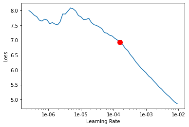
We are using the suggested learning rate above to train the model for 2000 epochs.
model.fit(100, lr=lr)| epoch | train_loss | valid_loss | accuracy | dice | time |
|---|---|---|---|---|---|
| 0 | 4.895883 | 2.304068 | 0.184192 | 0.133586 | 00:08 |
| 1 | 4.682844 | 2.228730 | 0.204355 | 0.134520 | 00:08 |
| 2 | 4.247415 | 2.247510 | 0.224069 | 0.164235 | 00:07 |
| 3 | 4.054215 | 2.261938 | 0.227853 | 0.208221 | 00:07 |
| 4 | 3.838150 | 2.207842 | 0.228400 | 0.144939 | 00:07 |
| 5 | 3.580566 | 2.180077 | 0.225253 | 0.128522 | 00:07 |
| 6 | 3.336041 | 2.150646 | 0.207254 | 0.175601 | 00:07 |
| 7 | 3.120762 | 2.073225 | 0.214026 | 0.152479 | 00:07 |
| 8 | 2.933001 | 2.045955 | 0.241302 | 0.153951 | 00:07 |
| 9 | 2.789467 | 2.084206 | 0.198224 | 0.173183 | 00:07 |
| 10 | 2.647619 | 1.934795 | 0.244913 | 0.174198 | 00:07 |
| 11 | 2.512081 | 1.907520 | 0.255222 | 0.159074 | 00:07 |
| 12 | 2.392307 | 1.823057 | 0.275607 | 0.213589 | 00:07 |
| 13 | 2.285432 | 1.765714 | 0.303430 | 0.194124 | 00:07 |
| 14 | 2.188699 | 1.735160 | 0.308035 | 0.242232 | 00:07 |
| 15 | 2.096217 | 1.696431 | 0.320136 | 0.239950 | 00:07 |
| 16 | 2.017443 | 1.629467 | 0.335706 | 0.289121 | 00:07 |
| 17 | 1.949237 | 1.587258 | 0.353876 | 0.290316 | 00:07 |
| 18 | 1.876262 | 1.538574 | 0.372055 | 0.330384 | 00:07 |
| 19 | 1.815327 | 1.527717 | 0.379276 | 0.334173 | 00:07 |
| 20 | 1.760807 | 1.603784 | 0.363623 | 0.307923 | 00:07 |
| 21 | 1.712551 | 1.464810 | 0.397946 | 0.327786 | 00:07 |
| 22 | 1.660718 | 1.420146 | 0.419562 | 0.373972 | 00:07 |
| 23 | 1.619952 | 1.407624 | 0.419846 | 0.358851 | 00:07 |
| 24 | 1.578108 | 1.363935 | 0.436551 | 0.396460 | 00:07 |
| 25 | 1.546720 | 1.382313 | 0.427362 | 0.350872 | 00:07 |
| 26 | 1.514228 | 1.343162 | 0.446262 | 0.406849 | 00:07 |
| 27 | 1.493786 | 1.349320 | 0.437524 | 0.355242 | 00:07 |
| 28 | 1.468180 | 1.318090 | 0.452631 | 0.403168 | 00:07 |
| 29 | 1.439874 | 1.293341 | 0.460748 | 0.407321 | 00:08 |
| 30 | 1.412643 | 1.312110 | 0.456506 | 0.394984 | 00:07 |
| 31 | 1.393659 | 1.298682 | 0.461176 | 0.413462 | 00:07 |
| 32 | 1.374351 | 1.285026 | 0.467914 | 0.433531 | 00:07 |
| 33 | 1.368896 | 1.271524 | 0.472473 | 0.411570 | 00:07 |
| 34 | 1.349091 | 1.257120 | 0.477335 | 0.420728 | 00:08 |
| 35 | 1.334518 | 1.237478 | 0.482465 | 0.434865 | 00:07 |
| 36 | 1.322255 | 1.229985 | 0.489380 | 0.445741 | 00:07 |
| 37 | 1.309935 | 1.218811 | 0.491339 | 0.449685 | 00:07 |
| 38 | 1.298364 | 1.241076 | 0.485703 | 0.440830 | 00:07 |
| 39 | 1.284544 | 1.206009 | 0.501767 | 0.467454 | 00:07 |
| 40 | 1.271894 | 1.195129 | 0.499503 | 0.465736 | 00:08 |
| 41 | 1.258210 | 1.204229 | 0.496341 | 0.447168 | 00:07 |
| 42 | 1.249108 | 1.188009 | 0.502429 | 0.482135 | 00:07 |
| 43 | 1.245222 | 1.205836 | 0.495398 | 0.459033 | 00:07 |
| 44 | 1.236919 | 1.166054 | 0.513800 | 0.482971 | 00:07 |
| 45 | 1.228589 | 1.172657 | 0.508676 | 0.458676 | 00:07 |
| 46 | 1.220988 | 1.183226 | 0.501324 | 0.438410 | 00:07 |
| 47 | 1.212198 | 1.190025 | 0.504303 | 0.455034 | 00:07 |
| 48 | 1.209525 | 1.182104 | 0.507495 | 0.457776 | 00:07 |
| 49 | 1.205935 | 1.161246 | 0.514066 | 0.464236 | 00:07 |
| 50 | 1.204263 | 1.152366 | 0.516409 | 0.475130 | 00:07 |
| 51 | 1.196822 | 1.176271 | 0.508255 | 0.481153 | 00:07 |
| 52 | 1.188036 | 1.146006 | 0.521011 | 0.488024 | 00:07 |
| 53 | 1.183094 | 1.153377 | 0.518954 | 0.489394 | 00:07 |
| 54 | 1.178807 | 1.135087 | 0.525720 | 0.492636 | 00:07 |
| 55 | 1.173015 | 1.144235 | 0.523340 | 0.496628 | 00:07 |
| 56 | 1.168650 | 1.138796 | 0.520963 | 0.467020 | 00:07 |
| 57 | 1.166994 | 1.148650 | 0.521436 | 0.477236 | 00:07 |
| 58 | 1.168930 | 1.126733 | 0.528690 | 0.486403 | 00:07 |
| 59 | 1.161723 | 1.112772 | 0.533466 | 0.504935 | 00:08 |
| 60 | 1.157561 | 1.119520 | 0.529660 | 0.491302 | 00:07 |
| 61 | 1.158854 | 1.139832 | 0.519275 | 0.486997 | 00:07 |
| 62 | 1.155192 | 1.113281 | 0.533511 | 0.493383 | 00:07 |
| 63 | 1.153943 | 1.121855 | 0.529218 | 0.483027 | 00:07 |
| 64 | 1.148564 | 1.149227 | 0.517923 | 0.475069 | 00:07 |
| 65 | 1.148768 | 1.112661 | 0.533261 | 0.487888 | 00:07 |
| 66 | 1.145626 | 1.116498 | 0.530466 | 0.487929 | 00:07 |
| 67 | 1.142795 | 1.106350 | 0.535092 | 0.491875 | 00:07 |
| 68 | 1.142005 | 1.109101 | 0.533545 | 0.502020 | 00:07 |
| 69 | 1.135479 | 1.111173 | 0.534888 | 0.491346 | 00:07 |
| 70 | 1.135544 | 1.104636 | 0.534119 | 0.497073 | 00:07 |
| 71 | 1.132466 | 1.102835 | 0.537323 | 0.496984 | 00:07 |
| 72 | 1.131976 | 1.097890 | 0.538928 | 0.503210 | 00:07 |
| 73 | 1.127540 | 1.099265 | 0.537723 | 0.500054 | 00:07 |
| 74 | 1.120606 | 1.093285 | 0.540417 | 0.503302 | 00:07 |
| 75 | 1.115077 | 1.097111 | 0.540237 | 0.504814 | 00:07 |
| 76 | 1.114371 | 1.092764 | 0.540207 | 0.505019 | 00:07 |
| 77 | 1.115887 | 1.094283 | 0.540009 | 0.504285 | 00:08 |
| 78 | 1.116468 | 1.099267 | 0.538202 | 0.502507 | 00:07 |
| 79 | 1.114179 | 1.088499 | 0.543567 | 0.514224 | 00:07 |
| 80 | 1.112337 | 1.090717 | 0.540167 | 0.504081 | 00:07 |
| 81 | 1.111818 | 1.092220 | 0.539713 | 0.498848 | 00:07 |
| 82 | 1.109563 | 1.086534 | 0.543723 | 0.508096 | 00:07 |
| 83 | 1.109317 | 1.086858 | 0.543741 | 0.508981 | 00:07 |
| 84 | 1.109809 | 1.090642 | 0.540866 | 0.499541 | 00:07 |
| 85 | 1.105921 | 1.085104 | 0.543176 | 0.507754 | 00:07 |
| 86 | 1.105818 | 1.085329 | 0.543622 | 0.510307 | 00:07 |
| 87 | 1.100395 | 1.088507 | 0.542453 | 0.508482 | 00:07 |
| 88 | 1.101971 | 1.083116 | 0.545029 | 0.511915 | 00:07 |
| 89 | 1.099825 | 1.082875 | 0.545221 | 0.512105 | 00:07 |
| 90 | 1.096118 | 1.083799 | 0.545013 | 0.512355 | 00:07 |
| 91 | 1.097838 | 1.083607 | 0.544434 | 0.510415 | 00:07 |
| 92 | 1.094332 | 1.082571 | 0.544855 | 0.510526 | 00:07 |
| 93 | 1.094872 | 1.084903 | 0.543506 | 0.506315 | 00:07 |
| 94 | 1.095193 | 1.083902 | 0.544208 | 0.507852 | 00:07 |
| 95 | 1.094048 | 1.085175 | 0.543402 | 0.505761 | 00:07 |
| 96 | 1.096176 | 1.084359 | 0.543930 | 0.506712 | 00:07 |
| 97 | 1.097573 | 1.084882 | 0.543655 | 0.508043 | 00:07 |
| 98 | 1.097415 | 1.085278 | 0.543436 | 0.507103 | 00:07 |
| 99 | 1.097319 | 1.084194 | 0.543799 | 0.506578 | 00:07 |
We have trained the model for a further 1900 epochs to improve model performance. For the sake of time, the cell below is commented out.
# model.fit(1900)Visualize classification results in validation set
It's a good practice to see results of the model vis-a-vis ground truth. The code below picks random samples and shows us ground truths and model predictions, side by side. This enables us to preview the results of the model within the notebook.
model.show_results()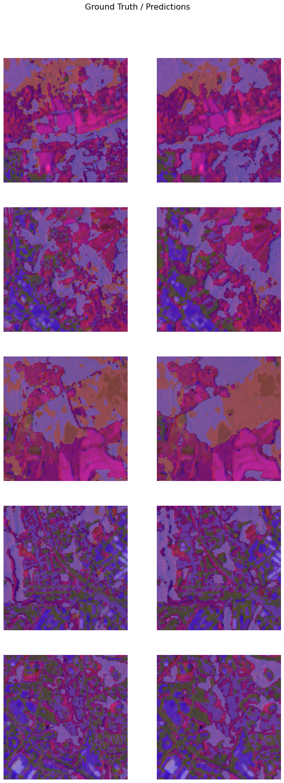
Evaluate model performance
As we have 7 classes for this segmentation task, we need to perform an accuracy assessment for each class. To achieve this, ArcGIS API for Python provides the per_class_metrics function that calculates a precision, recall, and f1 score for each class.
model.per_class_metrics()| NoData | Deciduous Forest | Developed, High Intensity | Developed, Low Intensity | Developed, Medium Intensity | Evergreen Forest | Mixed Forest | |
|---|---|---|---|---|---|---|---|
| precision | 0.689404 | 0.724823 | 0.772128 | 0.637362 | 0.637322 | 0.730950 | 0.600000 |
| recall | 0.738998 | 0.740948 | 0.782928 | 0.605665 | 0.645893 | 0.384463 | 0.415889 |
| f1 | 0.713340 | 0.732797 | 0.777490 | 0.621109 | 0.641579 | 0.503891 | 0.491261 |
Save model
We will save the model that we trained as a 'Deep Learning Package' ('.dlpk' format). A Deep Learning Package is the standard format used to deploy deep learning models on the ArcGIS platform.
We will use the save() method to save the trained model. By default, it will be saved to the 'models' sub-folder within our training data folder.
model.save('unet_2000e', publish=True, gis=gis)Computing model metrics...
WindowsPath('C:/data/2021/hyperspectral/hyperion_l8lulc_128px_64strd_30px_mask_frst_bltp_7classes/models/unet_2000e')Model inference
Using ArcGIS Pro, we can use the trained model on a test image/area to classify different types of built-up areas and forests in the hyperspectral satellite image.
After we have trained the UnetClassifier model and saved the weights for classifying images, we can use the Classify Pixels Using Deep Learning tool, available in both ArcGIS pro and ArcGIS Enterprise, for inferencing at scale.
inference_raster = ent_gis.content.get('a69ec3006c9a45a49b85cc43aa529e44')
inference_raster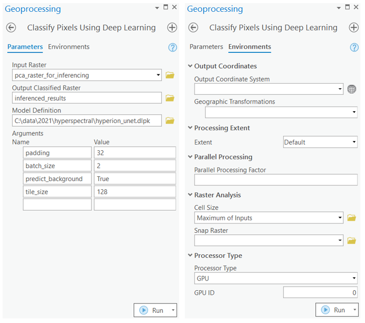
with arcpy.EnvManager(processorType="GPU"): out_classified_raster = arcpy.ia.ClassifyPixelsUsingDeepLearning("pca_raster_for_inferencing", r"C:\path\to\model.dlpk", "padding 32;batch_size 2;predict_background True; tile_size 128", "PROCESS_AS_MOSAICKED_IMAGE", None); out_classified_raster.save(r"C:\sample\sample.gdb\inferenced_results")
Results visualization
The classified output raster is generated using ArcGIS Pro. The output raster is published on the portal for visualization.
inferenced_results = ent_gis.content.get('03609691b9e74def954f81b9285dee93')
inferenced_resultsrgb_imagery = ent_gis.content.get('f9a5e23541b845da8846eb54ea561594')
rgb_imageryCreate map widgets
Two map widgets are created showing the RGB imagery and Inferenced results.
m1 = gis.map()
m1.content.add(rgb_imagery)
m1.basemap.basemap = 'satellite'
m2 = gis.map()
m2.content.add(inferenced_results)
Synchronize web maps
The maps are synchronized with each other using MapView.sync_navigation functionality. Map view synchronization helps in comparing the inferenced results with the RGB imagery. A detailed description about advanced map widget options can be referenced here.
m1.sync_navigation(m2)Set the map layout
from ipywidgets import HBox, VBox, Label, LayoutHbox and Vbox were used to set the layout of map widgets.
hbox_layout = Layout()
hbox_layout.justify_content = 'space-around'

hb1=HBox([Label('FCC imagery'),Label('Results')])
hb1.layout=hbox_layout
Results
The resulting predictions are provided as a map for better visualization.
VBox([hb1,HBox([m1,m2])])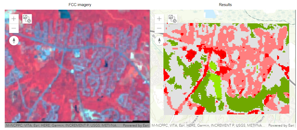
Inferenced results legend

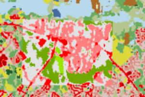
m2.zoom_to_layer(inferenced_results)In the map widgets, it can be seen that the model is able to differentiate between forests and open spaces (gardens, parks, etc). The different types of developed areas are also accurately classified by the model, with the bright blue-gray patches representing high density developed areas, for instance. The forested areas have also been accurately classified by the model.
Limitation
One of the major limitations in working with hyperspectral data is its lack of availability for many parts of the world. In comparison to multispectral imagery tiles, like those from Landsat-8, one tile of hyperion imagery covers a relatively small area. If a training dataset is prepared with multiple tiles, a model can be trained and more accurate results can be generated.
Conclusion
In this notebook, we have covered a lot of ground. In Part 1, we covered how Hyperion data can be downloaded using USGS Earth Explorer, the pre-processing steps of Hyperion, how to create a Principal Component raster, and how to export training data for deep learning using ArcGIS Pro. In Part 2, we demonstrated the steps to prepare the input data, train a pixel-based classification model, visualize the results, and generate the accuracy metrics. Finally, in Part 3, we demonstrated the process of inferencing results on a test raster/area. The same workflow can be used to identify minerals/rocks, plant species, oil spills, etc. using hyperspectral imageries and arcgis.learn models.
