- 🔬 Data Science
- 🥠 Deep Learning
Introduction
When ground data is not available, crater detection and counting play a vital role in predicting the moons surface age. Further, crater detection is necessary for identifying viable landing sites for lunar landers, as well as for establishing landmarks for navigation on the moon. Traditionally, craters have manually been digitized using visual interpretation, a very time-consuming and inefficient method. However, with the proliferation of deep learning, the process of crater detection is now able to be bolstered by automated detection. This notebook will demonstrate how the ArcGIS API for Python can be used to train a deep learning crater detection model using a Digital Elevation Model (DEM), which can then be deployed in ArcGIS Pro or ArcGIS Enterprise.
Necessary imports
import os
from pathlib import Path

from arcgis import GIS
from arcgis.learn import MaskRCNN, prepare_data
Connect to your GIS
gis = GIS('home')Export training data
The DEM of the moon will be used as input_raster for the training data and has a spatial resolution of 118m. It can be downloaded from the USGS website.
lunar_dem = gis.content.get('beae2f7947704c938eb957c6deb2fa2b')
lunar_demThe crater feature layer will be used as the Input Feature Class for the training data.
Feature layer of craters 5-20 km will be used to export training data at 500 and 5000 cell size.
craters_5_20km = gis.content.get('af240e45a3ca445b88d6ec19209d3bb5')
craters_5_20kmFeature layer of craters more than 20 km will be used to export training data at 10000 cell size.
craters_more_than_20km = gis.content.get('36272e93ec4547abba495c797a4fb921')
craters_more_than_20kmMethodology
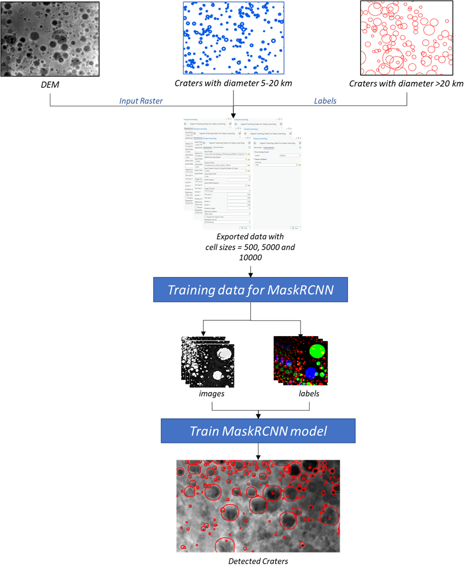
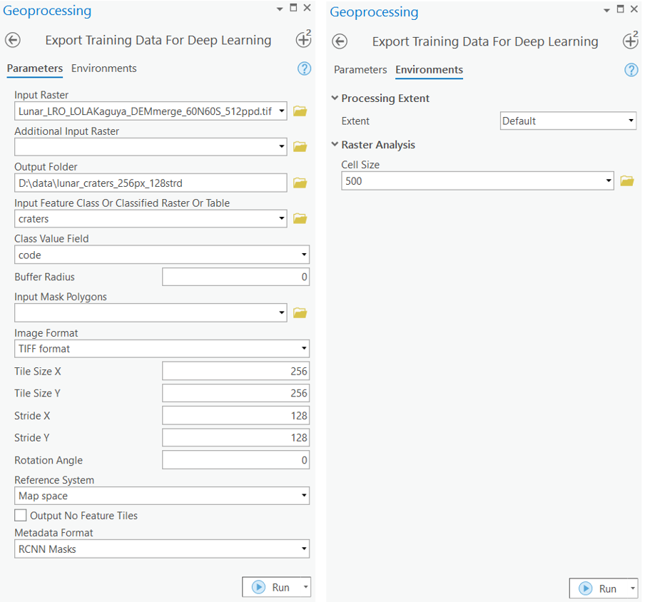
The data will be exported in the “RCNN Masks” metadata format, which is available in the Export Training Data For Deep Learning tool. This tool is available in both ArcGIS Pro and ArcGIS Image Server. The various inputs required by the tool are described below:
Input Raster: Lunar DEM
Input Feature Class Or Classified Raster Or Table: The craters feature layer
Tile Size X & Tile Size Y: 256
Stride X & Stride Y: 128
Meta Data Format: 'RCNN Masks', as we are training a MaskRCNN model.
Environments:
-
Cell Size: The data is exported to 3 different cell sizes so that it can learn to detect craters of different diameters. The data is exported at 500, 5000, and 10000. -
Processing Extent: Default
Note: The training data must be exported in the same output folder for all three cell sizes.
Inside the exported data folder, the 'images' folder contains all of the chips of the DEM, and the 'labels' folder contains the masks of the craters.
Model training
Alternatively, we have provided a subset of training data containing a few samples that follow the same directory structure mentioned above, as well as the raster and crater feature layers used for exporting the training dataset. The provided data can be used directly to run the experiments.
training_data = gis.content.get('0a4e2d4ad7bf41f6973c7e3434faf7d4')
training_datafilepath = training_data.download(file_name=training_data.name)#Extract the data from the zipped image collection
import zipfile
with zipfile.ZipFile(filepath, 'r') as zip_ref:
zip_ref.extractall(Path(filepath).parent)Prepare data
output_path = Path(os.path.join(os.path.splitext(filepath)[0]))data = prepare_data(output_path, batch_size=8)Visualize a few samples from your training data
To get a sense of what the training data looks like, the arcgis.learn.show_batch() method will randomly select a few training chips and visualize them.
data.show_batch(rows=2)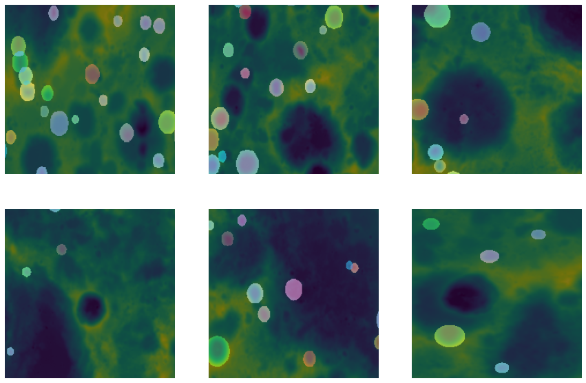
Load model architecture
The arcgis.learn module provides the MaskRCNN model for instance segmentation tasks. MaskRCNN is based on a pretrained convolutional neural network, like ResNet, that acts as the 'backbone'. More details about MaskRCNN can be found here.
model = MaskRCNN(data)Tuning for optimal learning rate
Learning rate is one of the most important hyperparameters in model training. ArcGIS API for Python provides a learning rate finder that automatically chooses the optimal learning rate for you.
lr = model.lr_find()
lr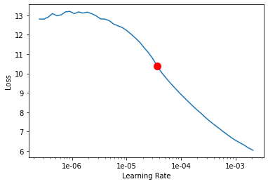
3.630780547701014e-05
Fit the model
Next, the model is trained for a few epochs, with early_stopping=True and the learning rate recommended above.
model.fit(100, lr, early_stopping=True)| epoch | train_loss | valid_loss | time |
|---|---|---|---|
| 0 | 6.944399 | 5.095363 | 01:00 |
| 1 | 3.083338 | 2.410944 | 01:04 |
| 2 | 2.264618 | 2.287425 | 01:08 |
| 3 | 2.102938 | 2.249945 | 01:09 |
| 4 | 2.032436 | 2.229557 | 01:15 |
| 5 | 2.009923 | 2.240452 | 01:15 |
| 6 | 1.982428 | 2.191599 | 01:12 |
| 7 | 1.960892 | 2.277536 | 01:17 |
| 8 | 1.991066 | 2.217761 | 01:17 |
| 9 | 1.938140 | 2.132267 | 01:17 |
| 10 | 1.868605 | 2.113236 | 01:19 |
| 11 | 1.777041 | 2.075418 | 01:17 |
| 12 | 1.724545 | 1.980257 | 01:17 |
| 13 | 1.688391 | 1.940772 | 01:17 |
| 14 | 1.644972 | 1.872948 | 01:16 |
| 15 | 1.611357 | 1.864072 | 01:14 |
| 16 | 1.533023 | 1.810667 | 01:17 |
| 17 | 1.539868 | 1.779850 | 01:18 |
| 18 | 1.511817 | 1.776860 | 01:19 |
| 19 | 1.489522 | 1.796499 | 01:18 |
| 20 | 1.478998 | 1.689595 | 01:17 |
| 21 | 1.482321 | 1.747638 | 01:16 |
| 22 | 1.459265 | 1.689370 | 01:15 |
| 23 | 1.395078 | 1.692547 | 01:13 |
| 24 | 1.419213 | 1.637439 | 01:15 |
| 25 | 1.407691 | 1.675853 | 01:13 |
| 26 | 1.384365 | 1.623085 | 01:13 |
| 27 | 1.354562 | 1.620516 | 01:21 |
| 28 | 1.345968 | 1.631758 | 01:13 |
| 29 | 1.368354 | 1.605378 | 01:13 |
| 30 | 1.350830 | 1.616508 | 01:13 |
| 31 | 1.324633 | 1.618946 | 01:12 |
| 32 | 1.297969 | 1.591982 | 01:12 |
| 33 | 1.263183 | 1.649768 | 01:13 |
| 34 | 1.288492 | 1.612240 | 01:13 |
| 35 | 1.299136 | 1.599925 | 01:12 |
| 36 | 1.276054 | 1.604237 | 01:12 |
| 37 | 1.261739 | 1.572726 | 01:12 |
| 38 | 1.270514 | 1.534423 | 01:13 |
| 39 | 1.265635 | 1.531221 | 01:15 |
| 40 | 1.278750 | 1.583697 | 01:15 |
| 41 | 1.257461 | 1.530308 | 01:13 |
| 42 | 1.254675 | 1.585197 | 01:13 |
| 43 | 1.251033 | 1.521029 | 01:13 |
| 44 | 1.240656 | 1.537336 | 01:13 |
| 45 | 1.257285 | 1.528091 | 01:13 |
| 46 | 1.228090 | 1.561426 | 01:22 |
| 47 | 1.197009 | 1.540503 | 01:15 |
| 48 | 1.249679 | 1.507996 | 01:17 |
| 49 | 1.214384 | 1.498527 | 01:14 |
| 50 | 1.208289 | 1.450118 | 01:15 |
| 51 | 1.200328 | 1.509240 | 01:13 |
| 52 | 1.184823 | 1.464436 | 01:19 |
| 53 | 1.176964 | 1.498307 | 01:15 |
| 54 | 1.203655 | 1.480856 | 01:14 |
| 55 | 1.156613 | 1.521594 | 01:14 |
Epoch 56: early stopping
Here, the model training automatically stopped at the 56th epoch. We can see reasonable results, as both the training and validation losses decreased considerably, indicating that the model is learning to translate between different domains of imagery.
Save the model
Here, we will save the trained model as a 'Deep Learning Package' ('.dlpk'). The Deep Learning Package format is the standard format used when deploying deep learning models on the ArcGIS platform.
model.save("moon_mrcnn_2", publish=True)Published DLPK Item Id: 81e635734e1b4d558cd51e2cee44833a
WindowsPath('C:/Users/shi10484/AppData/Local/Temp/lunar_craters_detection_from_digital_elevation_models_using_deep_learning/models/moon_mrcnn_2')Visualize results in validation set
It is a good practice to view the results of the model viz-a-viz the ground truth. The model.show_results() method can be used to display the detected craters. Each detection is visualized as a mask by default.
model.show_results(rows=2, mask_threshold=0.7)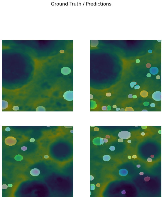
Accuracy assessment
For the accuracy assessment, we can compute the average precision score for the trained model. Average precision will compute the average precision on the validation set for each class. We can compute the average precision score by calling model.average_precision_score. It takes the following parameters:
detect_thresh: The probability above which a detection will be considered for computing the average precision.iou_thresh: The intersection over union threshold with the ground truth labels, above which a predicted bounding box will be considered a true positive.mean: If set toFalse, will return the class-wise average precision. Otherwise will return the mean average precision.
model.average_precision_score(){'1': 0.4536149187175708}Model inferencing
After training the MaskRCNN model and saving the weights of the detected crater masks, we can use the Detect Objects Using Deep Learning tool available in ArcGIS Pro and ArcGIS Image Server.
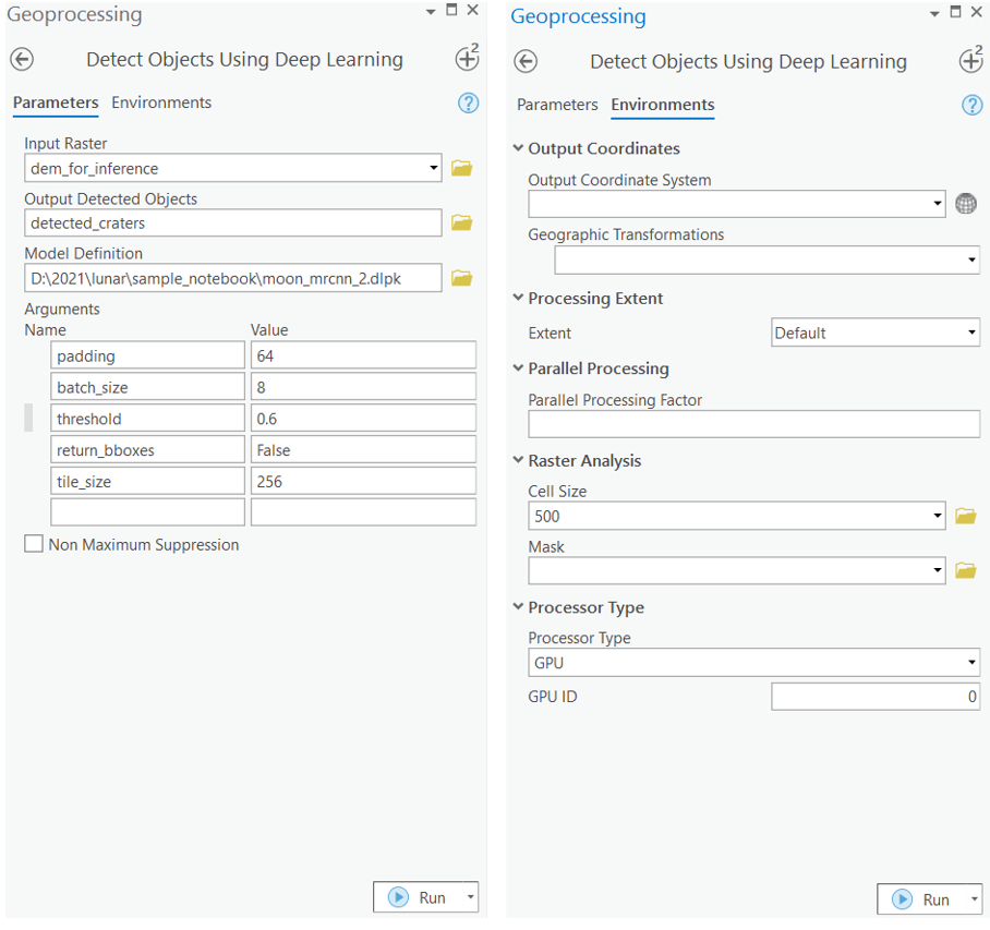
arcpy.ia.DetectObjectsUsingDeepLearning(in_raster="dem_for_inference", out_detected_objects=r"\\detected_craters", in_model_definition=r"\\models\moon_mrcnn_2\moon_mrcnn_2.dlpk", model_arguments ="padding 56;batch_size 4;threshold 0.6;return_bboxes False", run_nms="NMS", confidence_score_field="Confidence", class_value_field="Class", max_overlap_ratio=0, processing_mode="PROCESS_AS_MOSAICKED_IMAGE")
The inferencing above was done on the following cell sizes: 500m (small craters), 5000m (medium-sized craters), and 10,000m (large craters). All of the inferenced outputs were then merged together to get the final feature layer, which consists of all the detected craters.
Results visualization
Finally, after we have used ArcGIS Pro to detect craters in two different areas, we will publish the results to our portal and visualize them as maps.
from arcgis.map import Map
## Area1 Craters
LunarArea1 = gis.content.get('1a76ed548cfc4e159d860ae253e5ecc3')
map1 = Map(item=LunarArea1)
map1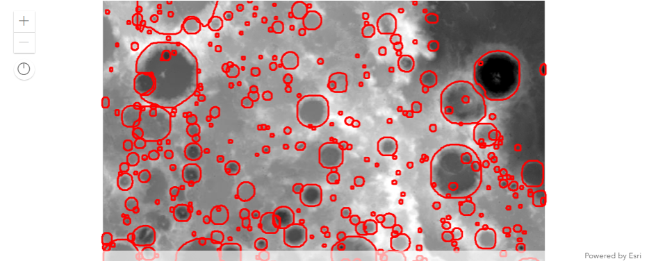
## Area2 Craters
LunarArea2 = gis.content.get('2ce5ad91fab649c7982dde750cce3390')
map2 = Map(item=LunarArea2)
map2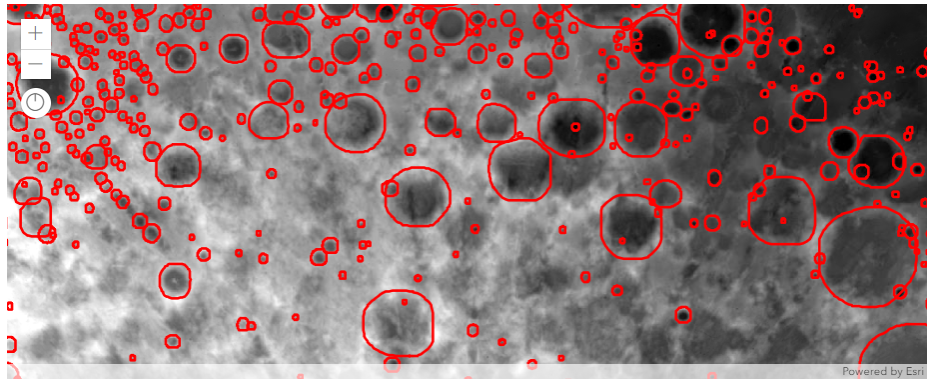
In the maps above, we can see that the trained MaskRCNN model was able to accurately detect craters of varying sizes. While the training data that was provided to the model contained craters digitized as circle features, the model was even able to learn to detect more accurate, non-circular boundaries of the craters.
Conclusion
This notebook showcased how instance segmentation models, like MaskRCNN, can be used to automatically detect lunar craters using a DEM. We also demonstrated how custom transformations based on the data, irrespective of already present standard transformations, can be added during data preparation to achieve better performance.

