- 🔬 Data Science
- 🥠 Deep Learning and Instance Segmentation
Introduction
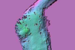
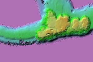
In this notebook, we will use bathymetry data provided by NOAA to detect shipwrecks from the Shell Bank Basin area located near New York City in United States. A Bathymetric Attributed Grid (BAG) is a two-band imagery where one of the bands is elevation and the other is uncertainty (define uncertainty of elevation value). We have applied deep learning methods after pre-processing the data (which is explained in Preprocess bathymetric data) for the detection.
One important step in pre-processing is applying shaded relief function provided in ArcGIS which is also used by NOAA in one of their BAG visualizations here. Shaded Relief is a 3D representation of the terrain which differentiate the shipwrecks distinctly from the background and reveals them. This is created by merging the Elevation-coded images and Hillshade method where a 3-band imagery is returned which is easy to interpret as compared to the raw bathymetry image. Subsequently, the images are exported as "RCNN Masks" to train a MaskRCNN model provided by ArcGIS API for Python for detecting the shipwrecks.
The notebook presents the use of deep learning methods to automate the identification of submerged shipwrecks which could be useful for hydrographic offices, archaeologists, historians who otherwise would spend a lot of time doing it manually.
Necessary imports
import os
from pathlib import Path
from datetime import datetime as dt

from arcgis.gis import GIS
from arcgis.raster.functions import RFT
from arcgis.learn import prepare_data, MaskRCNN
Connect to your GIS
gis = GIS('https://pythonapi.playground.esri.com/portal', 'arcgis_python', 'amazing_arcgis_123')Get the data for analysis
bathymetry_img = gis.content.get('8a08107910764b6d8418204800d3f8a4')
bathymetry_imgtraining_data_wrecks = gis.content.get('3384140ab9cc40a2ac0c41b71a9b4ec9')
training_data_wrecksPreprocess bathymetric data
We are applying some preprocessing to the bathymetry data so that we can export the data for training a deep learning model. The preprocessing steps include mapping 'No Data' pixels value to '-1' and applying Shaded Relief function to the output raster. The resultant raster after applying Shaded Relief function will be a 3-band imagery that we can use to export data using Export Training Data for Deep Learning tool in ArcGIS Pro 2.5, for training our deep learning model.
All the preprocessing steps are recorded in the form of a Raster function template which you can use in ArcGIS Pro to generate the processed raster.
shaded_relief_rft = gis.content.get('b0e3651e936e47f8bbf4144aea59e065')
shaded_relief_rftshaded_relief_ob = RFT(shaded_relief_rft)# ! conda install -c anaconda graphviz -y# shaded_relief_ob.draw_graph()
We need to add this custom raster function to ArcGIS Pro using Import functions option in the 'Custom' tab of 'Raster Functions'
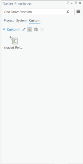
Once we apply the Raster function template on the bathymetry data, we will get the output image below. We will use this image to export training data for our deep learning model.
shaded_relief = gis.content.get('f09fd4cfcfae4dba860897a3d6d52926')
shaded_reliefExport training data
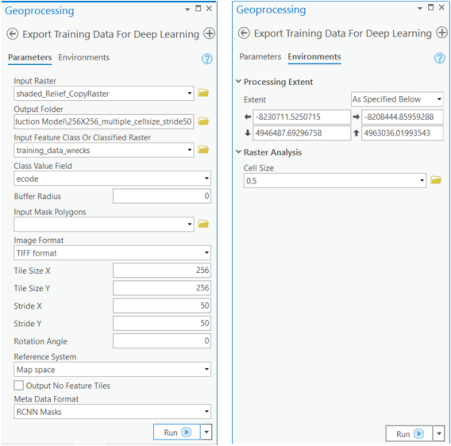
Export training data using 'Export Training data for deep learning' tool, click here for detailed documentation:
- Set 'shaded_relief' as
Input Raster. - Set a location where you want to export the training data in
Output Folderparameter, it can be an existing folder or the tool will create that for you. - Set the 'training_data_wrecks' as input to the
Input Feature Class Or Classified Rasterparameter. - Set
Class Field Valueas 'ecode'. - Set
Image Formatas 'TIFF format' Tile Size X&Tile Size Ycan be set to 256.Stride X&Stride Ycan be set to 50.- Select 'RCNN Masks' as the
Meta Data Formatbecause we are training a 'MaskRCNN Model'. - In 'Environments' tab set an optimum
Cell Size. For this example, as we have performing the analysis on the bathymetry data with 50 cm resolution, so, we used '0.5' as the cell size.
arcpy.ia.ExportTrainingDataForDeepLearning(in_raster="shaded_Relief_CopyRaster",
out_folder=r"\256X256_multiple_cellsize_stride50",
in_class_data="training_data_wrecks",
image_chip_format="TIFF",
tile_size_x=256,
tile_size_y=256,
stride_x=50,
stride_y=50,
output_nofeature_tiles="ONLY_TILES_WITH_FEATURES",
metadata_format="RCNN_Masks",
start_index=0,
class_value_field="ecode",
buffer_radius=0,
in_mask_polygons=None,
rotation_angle=0,
reference_system="MAP_SPACE",
processing_mode="PROCESS_AS_MOSAICKED_IMAGE",
blacken_around_feature="NO_BLACKEN",
crop_mode="FIXED_SIZE")```
Train the model
As we have already exported our training data, we will now train our model using ArcGIS API for Python. We will be using arcgis.learn module which contains tools and deep learning capabilities. Documentation is available here to install and setup environment.
Prepare data
We can always apply multiple transformations to our training data when training a model that can help generalize the model better. Though, we do some standard data augmentations, we can enhance them further based on the data at hand, to increase data size, and avoid occurring.
Let us have look, how we can do it using Fastai's image transformation library.
from fastai.vision.transform import crop, rotate, brightness, contrast, rand_zoomtrain_tfms = [rotate(degrees=30, # defining a transform using rotate with degrees fixed to
p=0.5), # a value, but by passing an argument p.
crop(size=224, # crop of the image to return image of size 224. The position
p=1., # is given by (col_pct, row_pct), with col_pct and row_pct
row_pct=(0, 1), # being normalized between 0 and 1.
col_pct=(0, 1)),
brightness(change=(0.4, 0.6)), # Applying change in brightness of image.
contrast(scale=(1.0, 1.5)), # Applying scale to contrast of image.
rand_zoom(scale=(1.,1.2))] # Randomized version of zoom.
val_tfms = [crop(size=224, # cropping the image to same size for validation datasets
p=1.0, # as in training datasets.
row_pct=0.5,
col_pct=0.5)]
transforms = (train_tfms, val_tfms) # tuple containing transformations for data augmentation
# of training and validation datasets respectively.We would specify the path to our training data and a few hyper parameters.
path: path of folder containing training data.batch_size: No of images your model will train on each step inside an epoch, it directly depends on the memory of your graphic card.transforms: tuple containing Fast.ai transforms for data augmentation of training and validation datasets respectively.
This function will return a fast.ai databunch, we will use this in the next step to train a model.
gis = GIS('home')training_data = gis.content.get('91178e9303af49b0b9ae09c0d32ec164')
training_datafilepath = training_data.download(file_name=training_data.name)import zipfile
with zipfile.ZipFile(filepath, 'r') as zip_ref:
zip_ref.extractall(Path(filepath).parent)data_path = Path(os.path.join(os.path.splitext(filepath)[0]))data = prepare_data(path=data_path, batch_size=8, transforms=transforms)Visualize a few samples from your training data
To make sense of training data we will use the show_batch() method in arcgis.learn. This method randomly picks few samples from the training data and visualizes them.
rows: number of rows we want to see the results for.
data.show_batch(rows=5)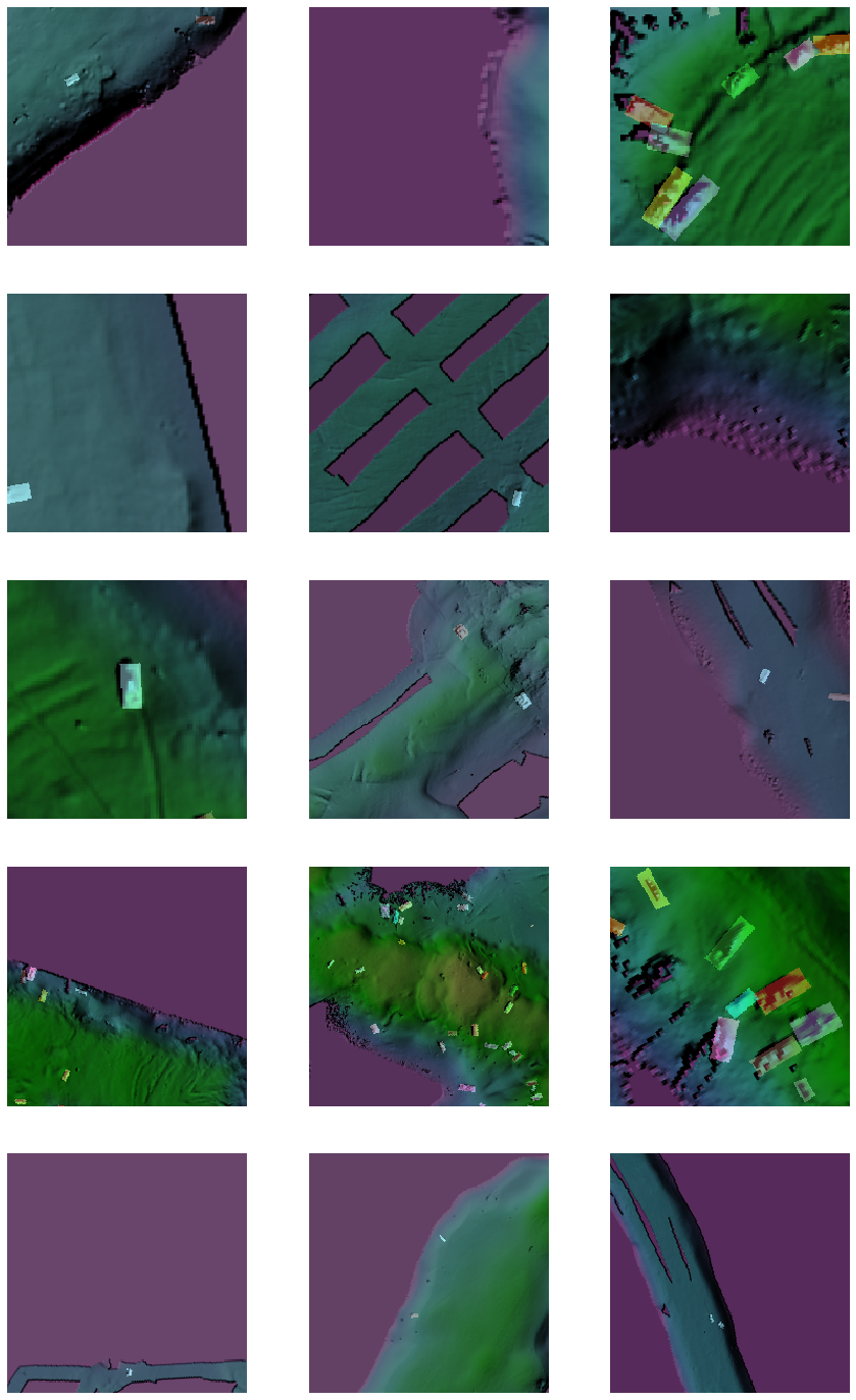
Load model architecture
arcgis.learn provides the MaskRCNN model for instance segmentation tasks, which is based on a pretrained convnet, like ResNet that acts as the 'backbone'. More details about MaskRCNN can be found here.
model = MaskRCNN(data)Find an optimal learning rate
Learning rate is one of the most important hyperparameters in model training. Here, we explore a range of learning rate to guide us to choose the best one. We will use the lr_find() method to find an optimum learning rate at which we can train a robust model.
lr = model.lr_find()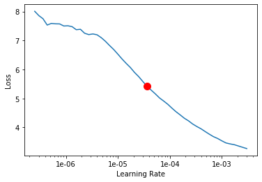
3.630780547701014e-05
Fit the model
To train the model, we use the fit() method. To start, we will train our model for 80 epochs. Epoch defines how many times model is exposed to entire training set. We have passes three parameters to fit() method:
epochs: Number of cycles of training on the data.lr: Learning rate to be used for training the model.wd: Weight decay to be used.
model.fit(epochs=80, lr=lr, wd=0.1)| epoch | train_loss | valid_loss | time |
|---|---|---|---|
| 0 | 0.883735 | 0.902166 | 56:25 |
| 1 | 0.814753 | 0.846428 | 58:18 |
| 2 | 0.780305 | 0.805268 | 57:48 |
| 3 | 0.732431 | 0.769769 | 53:34 |
| 4 | 0.692594 | 0.739427 | 47:35 |
| 5 | 0.656296 | 0.697303 | 57:13 |
| 6 | 0.605197 | 0.665202 | 43:11 |
| 7 | 0.609203 | 0.635087 | 43:09 |
| 8 | 0.582312 | 0.608184 | 43:13 |
| 9 | 0.569569 | 0.597905 | 43:17 |
| 10 | 0.542924 | 0.572707 | 43:30 |
| 11 | 0.544635 | 0.547287 | 54:32 |
| 12 | 0.520006 | 0.548388 | 55:43 |
| 13 | 0.500081 | 0.536543 | 57:37 |
| 14 | 0.511551 | 0.526891 | 57:28 |
| 15 | 0.492752 | 0.524570 | 58:10 |
| 16 | 0.475508 | 0.520521 | 58:07 |
| 17 | 0.495050 | 0.509737 | 57:58 |
| 18 | 0.479058 | 0.500814 | 58:06 |
| 19 | 0.472825 | 0.501527 | 58:05 |
| 20 | 0.458631 | 0.484302 | 58:17 |
| 21 | 0.478841 | 0.504961 | 52:08 |
| 22 | 0.456699 | 0.472860 | 49:15 |
| 23 | 0.439140 | 0.475529 | 57:53 |
| 24 | 0.431907 | 0.480451 | 57:59 |
| 25 | 0.441682 | 0.469926 | 58:14 |
| 26 | 0.432539 | 0.471899 | 58:36 |
| 27 | 0.420269 | 0.463864 | 58:15 |
| 28 | 0.428666 | 0.456262 | 58:31 |
| 29 | 0.405511 | 0.469793 | 58:14 |
| 30 | 0.418783 | 0.450741 | 59:26 |
| 31 | 0.400144 | 0.456605 | 58:34 |
| 32 | 0.427380 | 0.449641 | 56:08 |
| 33 | 0.404402 | 0.448000 | 47:59 |
| 34 | 0.403671 | 0.447599 | 57:55 |
| 35 | 0.388911 | 0.448730 | 58:26 |
| 36 | 0.415838 | 0.440210 | 58:16 |
| 37 | 0.402994 | 0.440201 | 58:21 |
| 38 | 0.374895 | 0.433149 | 58:23 |
| 39 | 0.385291 | 0.434547 | 58:14 |
| 40 | 0.390463 | 0.432285 | 58:18 |
| 41 | 0.370466 | 0.427367 | 58:03 |
| 42 | 0.395430 | 0.445681 | 58:21 |
| 43 | 0.367967 | 0.429725 | 58:06 |
| 44 | 0.372946 | 0.426311 | 47:39 |
| 45 | 0.376778 | 0.428242 | 53:26 |
| 46 | 0.378003 | 0.422538 | 57:56 |
| 47 | 0.392606 | 0.425642 | 58:30 |
| 48 | 0.374920 | 0.412655 | 57:56 |
| 49 | 0.381698 | 0.415867 | 58:11 |
| 50 | 0.366353 | 0.416311 | 57:48 |
| 51 | 0.377435 | 0.407092 | 58:35 |
| 52 | 0.370788 | 0.410003 | 58:43 |
| 53 | 0.393365 | 0.410419 | 58:21 |
| 54 | 0.355197 | 0.406449 | 58:09 |
| 55 | 0.359474 | 0.405332 | 54:09 |
| 56 | 0.357601 | 0.404893 | 48:12 |
| 57 | 0.366775 | 0.400052 | 58:24 |
| 58 | 0.358649 | 0.398841 | 58:31 |
| 59 | 0.344561 | 0.398987 | 59:00 |
| 60 | 0.361493 | 0.401714 | 58:18 |
| 61 | 0.352309 | 0.390297 | 58:27 |
| 62 | 0.342283 | 0.395422 | 58:41 |
| 63 | 0.341592 | 0.392883 | 59:12 |
| 64 | 0.361798 | 0.392384 | 58:28 |
| 65 | 0.350822 | 0.390853 | 58:33 |
| 66 | 0.348730 | 0.383924 | 58:35 |
| 67 | 0.342895 | 0.383599 | 48:18 |
| 68 | 0.341520 | 0.384532 | 44:22 |
| 69 | 0.339722 | 0.385112 | 43:54 |
| 70 | 0.341795 | 0.384323 | 43:48 |
| 71 | 0.349706 | 0.383976 | 43:54 |
| 72 | 0.326755 | 0.381668 | 43:45 |
| 73 | 0.325312 | 0.381942 | 43:54 |
| 74 | 0.335486 | 0.381422 | 43:43 |
| 75 | 0.345488 | 0.381084 | 43:56 |
| 76 | 0.343328 | 0.381468 | 43:54 |
| 77 | 0.326794 | 0.381019 | 44:05 |
| 78 | 0.333449 | 0.380597 | 44:00 |
| 79 | 0.338054 | 0.380587 | 43:51 |
As you can see, both the losses (valid_loss and train_loss) started from a higher value and ended up to a lower value, that tells our model has learnt well. Let us do an accuracy assessment to validate our observation.
Accuracy Assessment
We can compute the average precision score for the model we just trained in order to do the accuracy assessment. Average precision computes average precision on the validation set for each class. We can compute the Average Precision Score by calling model.average_precision_score. It takes the following parameters:
detect_thresh: The probability above which a detection will be considered for computing average precision.iou_thresh: The intersection over union threshold with the ground truth labels, above which a predicted bounding box will be considered a true positive.mean: If False, returns class-wise average precision otherwise returns mean average precision.
model.average_precision_score(detect_thresh=0.3, iou_thresh=0.3, mean=False){'1': 0.9417281930692071}The model has an average precision score of 0.94 which proves that the model has learnt well. Let us now see it's results on validation set.
Visualize results in validation set
The code below will pick a few random samples and show us ground truth and respective model predictions side by side. This allows us to validate the results of your model in the notebook itself. Once satisfied we can save the model and use it further in our workflow. The model.show_results() method can be used to display the detected ship wrecks. Each detection is visualized as a mask by default.
model.show_results(rows=5, thresh=0.5)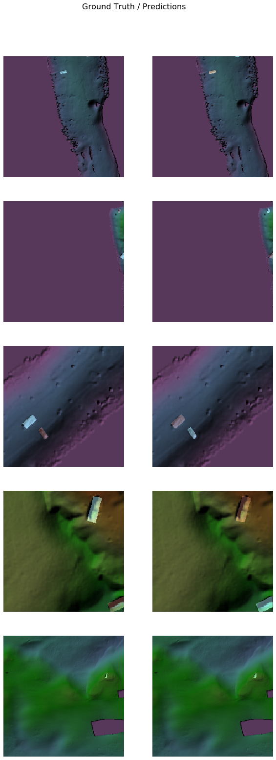
Save the model
We would now save the model which we just trained as a 'Deep Learning Package' or '.dlpk' format. Deep Learning package is the standard format used to deploy deep learning models on the ArcGIS platform.
We will use the save() method to save the model and by default it will be saved to a folder 'models' inside our training data folder itself.
model.save('Shipwrecks_80e')The saved model can be downloaded from here for inferencing purposes.
Model inference
The saved model can be used to detect shipwrecks masks using the Detect Objects Using Deep Learning tool available in ArcGIS Pro, or ArcGIS Image Server. For this sample, we will use the bathymetry data processed using the shaded relief raster function template to detect shipwrecks.
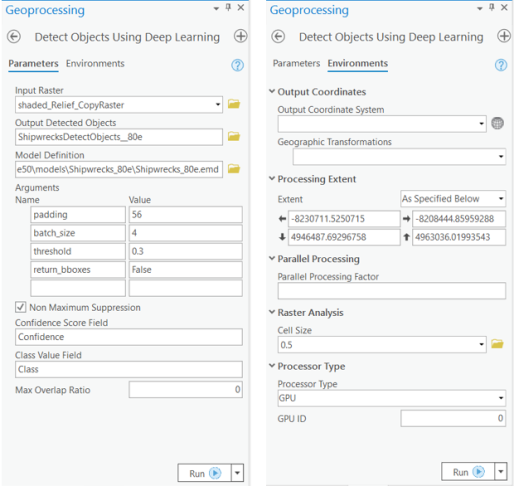
arcpy.ia.DetectObjectsUsingDeepLearning(in_raster="shaded_Relief_CopyRaster",
out_detected_objects=r"\\ShipwrecksDetectObjects_80e",
in_model_definition=r"\\models\Shipwrecks_80e\Shipwrecks_80e.emd",
model_arguments ="padding 56;batch_size 4;threshold 0.3;return_bboxes False",
run_nms="NMS",
confidence_score_field="Confidence",
class_value_field="Class",
max_overlap_ratio=0,
processing_mode="PROCESS_AS_MOSAICKED_IMAGE")
The output of the model is a layer of detected shipwrecks which is shown below:
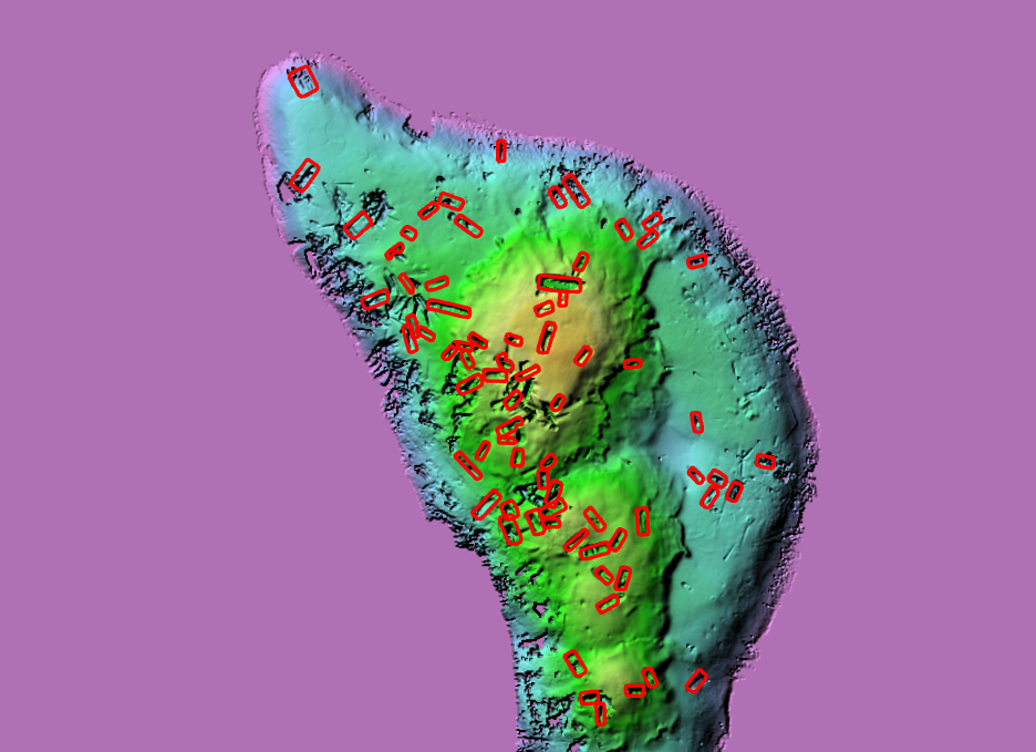
A subset of detected shipwrecks
To view the above results in a webmap click here.
Conclusion
This notebook showcased how instance segmentation models like MaskRCNN can be used to automatically detect shipwrecks using bathymetry data. This notebook also showcased how custom transformations, irrespective of already present standard transformations, based on the data, can be added while preparing data in order to achieve better performance.
