Introduction
Deep Learning models are huge and requires high computation for inferencing. Can we train Deep Learning models which require less computation power, are smaller in size and can be deployed on mobile phones? Well, the answer is 'yes'. With the integration of capability to train TensorFlow lite models with ArcGIS API for Python, we can now train DL models that can be deployed on mobile devices and are smaller in size.
Where can we use them? We can use them up to train multiple DL models to perform classification tasks specifically for mobile devices. One such integration we did is in the "Survey123" application which is a simple and intuitive form-centric data gathering solution being used by multiple surveyors while performing ground surveys, where we integrated a tf-lite model to classify different plant species while clicking it's picture in the app.
This notebook intends to showcase this capability to train a deep learning model that can be used in mobile applications for a real time inferencing using TensorFlow Lite framework. As an example, we will train the same plant species classification model which was discussed earlier but with a smaller dataset.
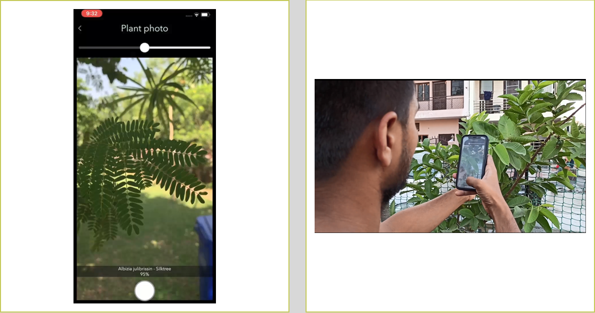
A snapshot of plant classifier in Survey123 application
Get the data for analysis
PlantCLEF data is available in three sets:
- a “trusted” training set based on the online collaborative Encyclopedia Of Life (EoL) [1].
- A ”noisy” training set (obtained from Google and Bing image search results, including mislabeled or irrelevant images [2].
- The previous years (2015-2016) images depicting only a subset of the species [3].
For this notebook, we have taken a subset from the "trusted" training set based on the online collaborative Encyclopedia Of Life [1] with 39,354 images belonging to 100 plant species and changed their specie numbers with specie names, as an example specie number '42' is changed to 'Acanthus mollis'. The information about the specie name is present in the "xml" file present along with each image file. We wrote a script to perform the specie name and specie number mapping. To know how we have done this, please have a look at the script here.
Use the following command to run the downloaded script. It requires three arguments to be passed:
- path to downloaded PlantCLEF data
- path of the destination folder
python changing_specie_name_with_number.py data/path dest/path
Train an image classification model
We will train our model using arcgis.learn module within ArcGIS API for Python. arcgis.learn contains tools and deep learning capabilities required for this study. A detailed documentation to install and setup the environment is available here.
Necessary imports
Firstly, we need to set the environment variable for ArcGIS to enable TensorFlow as backend. To perform this, we can set ARCGIS_ENABLE_TF_BACKEND parameter's value to 1 as shown below.
%env ARCGIS_ENABLE_TF_BACKEND=1env: ARCGIS_ENABLE_TF_BACKEND=1
import os
from pathlib import Path

from arcgis.gis import GIS
from arcgis.learn import prepare_data, FeatureClassifier
Download Dataset
gis = GIS('home')training_data = gis.content.get('81932a51f77b4d2d964218a7c5a4af17')
training_datafilepath = training_data.download(file_name=training_data.name)import zipfile
with zipfile.ZipFile(filepath, 'r') as zip_ref:
zip_ref.extractall(Path(filepath).parent)data_path = Path(os.path.join(os.path.splitext(filepath)[0]))Filter out non RGB Images
from glob import glob
from PIL import Image
for image_filepath in glob(os.path.join(data_path, 'images', '**','*.jpg')):
if Image.open(image_filepath).mode != 'RGB':
os.remove(image_filepath)Prepare data
We will now use the prepare_data() function to apply various types of transformations and augmentations on the training data. These augmentations enable us to train a better model with limited data and also prevent the model from overfitting.
Here, we are passing 3 parameters to the prepare_data() function.
path: path of folder containing training data.chip_size: Same as per specified while exporting training data.batch_size: No. of images your model will train on each step inside an epoch, it directly depends on the memory of your graphic card and the type of model which you are working with. For this sample, a batch size of 64 worked for us on a GPU with 11GB memory.
data = prepare_data(
    path=data_path,
    dataset_type='Imagenet',
    batch_size=64,
    chip_size=300
)
Visualize a few samples from your training data
To make sense of training data we will use the show_batch() method in arcgis.learn. show_batch() randomly picks a few samples from the training data and visualizes them.
rows: No of rows we want to see the results for.
data.show_batch(rows=2)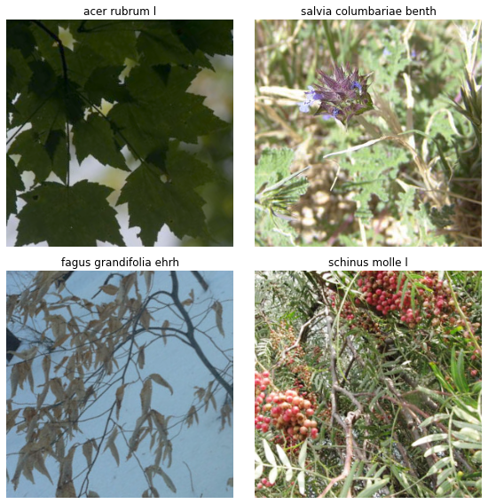
Load model architecture
arcgis.learn provides capabilities to determine class of each feature in the form of FeatureClassifier model. To have an in-depth information about it's working and usage, have a look at this link.
As we are training a model to be deployed on mobile phones, we must define the model with "tensorflow" backend. In order to do that we can set the parameter backend to "tensorflow".
model = FeatureClassifier(data, backbone='MobileNetV2', backend='tensorflow')Find an optimal learning rate
Learning rate is one of the most important hyperparameters in model training. Here, we explore a range of learning rates to guide us to choose the best one. arcgis.learn leverages fast.ai’s learning rate finder to find an optimum learning rate for training models. We can use the lr_find() method to find the optimum learning rate at which can train a robust model fast enough.
lr = model.lr_find()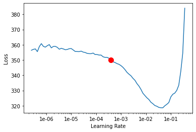
0.00039810716
Based on the learning rate plot above, we can see that the learning rate suggested by lr_find() for our training data is 0.000691831. We can use it to train our model. In the latest release of arcgis.learn we can train models without even specifying a learning rate. That internally uses the learning rate finder to find an optimal learning rate and uses it.
Fit the model
To train the model, we use the fit() method. To start, we will use 25 epochs to train our model. Epoch defines how many times model is exposed to entire training set.
model.fit(25, lr=lr)| epoch | train_loss | valid_loss | time |
|---|---|---|---|
| 0 | 282.509796 | 284.545929 | 06:33 |
| 1 | 219.822098 | 216.609177 | 06:11 |
| 2 | 184.608017 | 179.594299 | 06:16 |
| 3 | 157.201462 | 152.107513 | 06:13 |
| 4 | 146.833130 | 143.230316 | 06:08 |
| 5 | 142.532150 | 140.502411 | 06:06 |
| 6 | 130.854355 | 128.107193 | 06:13 |
| 7 | 123.135384 | 120.282646 | 06:16 |
| 8 | 122.825447 | 121.192963 | 06:15 |
| 9 | 113.097366 | 110.876205 | 06:09 |
| 10 | 110.630867 | 107.839455 | 06:05 |
| 11 | 105.668732 | 102.160103 | 06:08 |
| 12 | 104.367531 | 101.760544 | 06:11 |
| 13 | 96.982460 | 92.826294 | 06:10 |
| 14 | 94.381241 | 90.038216 | 06:11 |
| 15 | 91.442261 | 87.211021 | 06:12 |
| 16 | 89.456108 | 84.471718 | 06:19 |
| 17 | 88.846085 | 85.127541 | 06:02 |
| 18 | 85.060516 | 80.282585 | 06:05 |
| 19 | 83.723434 | 80.030220 | 06:20 |
| 20 | 82.750427 | 78.108757 | 06:26 |
| 21 | 81.436134 | 77.348999 | 06:27 |
| 22 | 80.915581 | 77.150444 | 06:26 |
| 23 | 81.231522 | 77.088852 | 06:26 |
| 24 | 80.637024 | 76.966454 | 06:26 |
Visualize results in validation set
The code below will pick a few random samples and show us ground truth and respective model predictions side by side. This allows us to validate the results of your model in the notebook itself. Once satisfied, we can save the model and use it further in our workflow.
model.show_results(rows=4, thresh=0.2)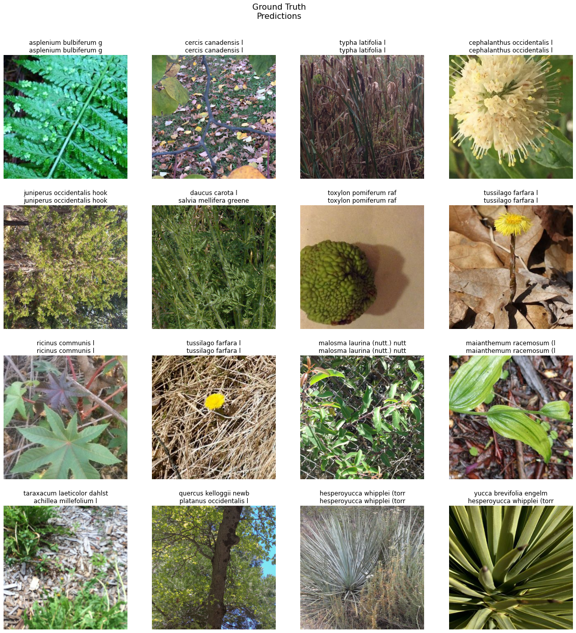
Here a subset of ground truth from training data is visualized along with the predictions from the model. As we can see, our model is performing well and the predictions are comparable to the ground truth.
Save the model
We will save the model which we trained in a tf-lite format.
We will use the save() method to save the trained model. By default, it will be saved to the 'models' sub-folder within our training data folder.
model.save('Plant-identification-25-tflite', framework="tflite")Deploy model
The tf-lite model can now be deployed on mobile devices. ArcGIS Survey123 app supports tf-lite models. For more information see Smart Assistants
References
[1] http://otmedia.lirmm.fr/LifeCLEF/PlantCLEF2017/TrainPackages/PlantCLEF2017Train1EOL.tar.gz
[2] http://otmedia.lirmm.fr/LifeCLEF/PlantCLEF2017/TrainPackages/PlantCLEF2017Train2Web.txt
[3] http://otmedia.lirmm.fr/LifeCLEF/PlantCLEF2015/Packages/TrainingPackage/PlantCLEF2015TrainingData.tar.gz
