- 🔬 Data Science
- 🥠 Deep Learning and pixel classification
Introduction
Flooding is one of the most frequent and costly forms of natural disasters. They often strike without warning and can occur when large volumes of water fall in a short time, causing flash floods. Flood mapping is typically performed using the following methods:
- Aerial observations
- Ground surveys
However, when flooding is widespread, these methods become prohibitively expensive and time consuming. Furthermore, aerial observation and optical imagery can often prove difficult, if not impossible, due to obstructive weather conditions. During flooding conditions, clouds can prevent the use of optical satellite imagery for visualization and analysis. In these instances, synthetic-aperture radar (SAR) allows us to penetrate through clouds and hazy atmospheric conditions to continuously observe and map flooding.
In 2019, severe flooding occurred in the Midwest of the United States. Also known as the Great Flood of 2019, 14 million people were affected across multiple states. In this analysis, we will perform flood mapping and infrastructural inundation mapping of the St. Peters region of Missouri, which was one of the affected areas during the flood.
Necessary imports
import os
from datetime import datetime
from pathlib import Path

from arcgis.gis import GIS
from arcgis.learn import prepare_data, UnetClassifier
from arcgis.raster import Raster, convert_raster_to_feature
from arcgis.features.manage_data import overlay_layers
from arcgis.features.analysis import dissolve_boundaries
Connect to your GIS
from arcgis import GIS
gis = GIS('home')
gis_ent = GIS(profile='your_enterprise_profile')
Export training data
Here, we convert the Sentinel-1 GRD VH polarization band to a 3 band raster using Export Raster. Under the Render Settings section, once Use Renderer is checked, Force RGB will be enabled.

The resulting raster is generated from the Sentinel-1 GRD VH imagery using traditional histogram thresholding technique. The raster contains two classes, permanent waterbodies and flood water. This raster will be used as a Classified Raster in the Export Training Data Using Deep Learning tool.
input_raster = gis_ent.content.get("ca56c6a8be4b44efad2b5fcec25270b2")
input_rasterThe feature layer contains two classes: 1 = Permanent Waterbodies and 2 = Flood Water. The feature layer will be used as the Input Feature Class in the Export Training Data For Deep Learning tool.
label_raster = gis_ent.content.get("2d52064d4eb54559b75ff4451cb6d52b")
label_rasterThe polygon feature class will be used as Input Mask Polygons in the Export Training Data For Deep Learning tool to delineate the area where image chips will be created.
aoi = gis_ent.content.get("d378a12e00a24815a306965e1917601d")
aoiThe Export Training Data For Deep Learning tool is used to prepare training data for training a deep learning model. The tool is available in both ArcGIS Pro and ArcGIS Enterprise.
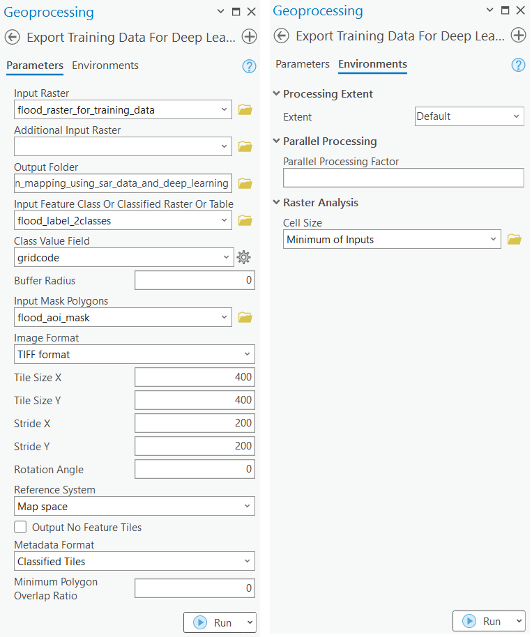
Next, we will utilize Jupyter Notebooks. Documentation on how to install and setup the necessary environment is available here.
Model training
Get training data
We have already exported the data, and it can be directly downloaded using the following steps:
training_data = gis.content.get('c4f58fd8e21743d69c82a93b30c8b873')
training_datafilepath = training_data.download(file_name=training_data.name)import zipfile
with zipfile.ZipFile(filepath, 'r') as zip_ref:
zip_ref.extractall(Path(filepath).parent)data_path = Path(os.path.join(os.path.splitext(filepath)[0]))Prepare data
The prepare_data function takes a training data path as input and creates a fast.ai databunch with specified parameters, like transformation, batch size, split percentage, etc.
data = prepare_data(data_path, batch_size=4, chip_size=400)Visualize training data
To get a sense of what the training data looks like, the arcgis.learn.show_batch() method will randomly select a few training chips and visualize them.
data.show_batch(rows=3)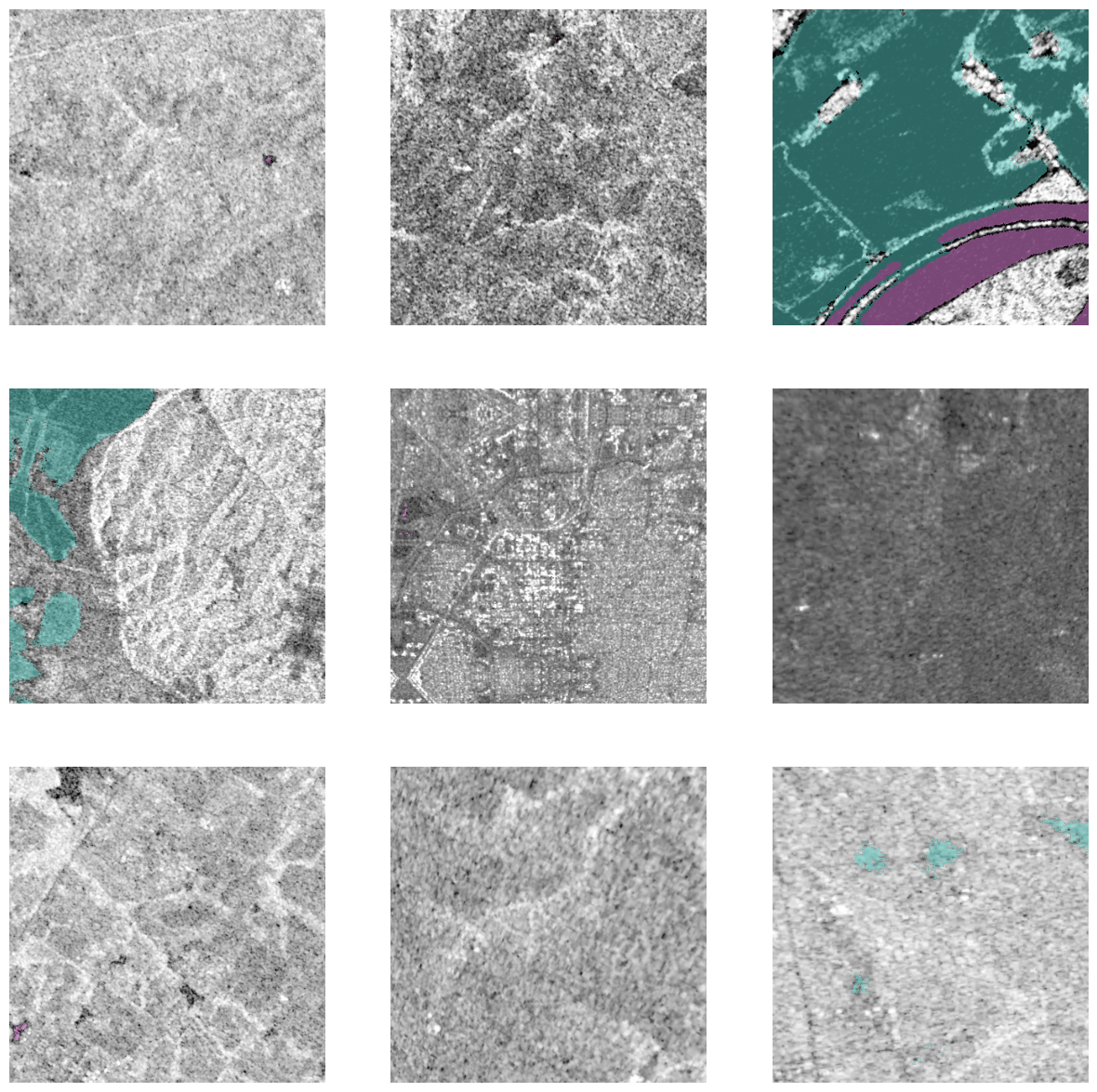
Load model architecture
arcgis.learn provides the UnetClassifier model for per pixel classification that is based on a pretrained convnet, like ResNet, that acts as the backbone. More details about UnetClassifier can be found here.
# Create U-Net Model
unet = UnetClassifier(data, backbone='resnet34')unet.unfreeze()Train the model
lr = unet.lr_find()
lr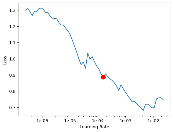
0.0001584893192461114
We are using the suggested learning rate above to train the model for 400 epochs.
unet.fit(100, lr=lr)| epoch | train_loss | valid_loss | accuracy | dice | time |
|---|---|---|---|---|---|
| 0 | 0.056524 | 0.064984 | 0.976062 | 0.608772 | 06:45 |
| 1 | 0.062250 | 0.065558 | 0.976453 | 0.596853 | 03:28 |
| 2 | 0.054321 | 0.065829 | 0.974905 | 0.606779 | 03:29 |
| 3 | 0.055470 | 0.065657 | 0.975155 | 0.612507 | 03:38 |
| 4 | 0.057925 | 0.062683 | 0.975891 | 0.612544 | 03:41 |
| 5 | 0.046697 | 0.066485 | 0.975312 | 0.612030 | 03:38 |
| 6 | 0.048388 | 0.067163 | 0.974090 | 0.605625 | 03:34 |
| 7 | 0.057085 | 0.068184 | 0.974643 | 0.599440 | 03:37 |
| 8 | 0.057320 | 0.063318 | 0.976909 | 0.601846 | 03:39 |
| 9 | 0.055874 | 0.064139 | 0.976454 | 0.618239 | 03:39 |
| 10 | 0.059982 | 0.065377 | 0.975455 | 0.604646 | 03:34 |
| 11 | 0.064432 | 0.062893 | 0.975681 | 0.603195 | 03:30 |
| 12 | 0.052742 | 0.067008 | 0.975461 | 0.591229 | 03:34 |
| 13 | 0.060652 | 0.065659 | 0.975032 | 0.553587 | 03:39 |
| 14 | 0.067467 | 0.078193 | 0.971295 | 0.611042 | 03:33 |
| 15 | 0.046704 | 0.068864 | 0.974196 | 0.565879 | 03:34 |
| 16 | 0.056145 | 0.070627 | 0.974419 | 0.602660 | 03:31 |
| 17 | 0.066529 | 0.081896 | 0.969127 | 0.601966 | 03:32 |
| 18 | 0.063344 | 0.068490 | 0.974117 | 0.600837 | 03:32 |
| 19 | 0.072548 | 0.073396 | 0.972721 | 0.619006 | 03:29 |
| 20 | 0.061560 | 0.074958 | 0.972994 | 0.613835 | 03:33 |
| 21 | 0.060021 | 0.068872 | 0.974412 | 0.615664 | 03:28 |
| 22 | 0.060153 | 0.072947 | 0.973799 | 0.592877 | 03:29 |
| 23 | 0.076432 | 0.086417 | 0.968766 | 0.583267 | 03:32 |
| 24 | 0.084845 | 0.076841 | 0.973072 | 0.583452 | 03:28 |
| 25 | 0.064284 | 0.065808 | 0.975677 | 0.557439 | 03:29 |
| 26 | 0.069426 | 0.069917 | 0.973683 | 0.616697 | 03:29 |
| 27 | 0.066233 | 0.076777 | 0.970253 | 0.616763 | 03:28 |
| 28 | 0.061531 | 0.069077 | 0.974110 | 0.615580 | 03:28 |
| 29 | 0.059284 | 0.073190 | 0.973690 | 0.542749 | 03:28 |
| 30 | 0.065980 | 0.069973 | 0.976707 | 0.608508 | 03:29 |
| 31 | 0.070354 | 0.092594 | 0.966464 | 0.551362 | 03:30 |
| 32 | 0.072470 | 0.093456 | 0.965545 | 0.591326 | 03:31 |
| 33 | 0.062519 | 0.069911 | 0.975124 | 0.541391 | 03:33 |
| 34 | 0.064994 | 0.067970 | 0.975051 | 0.575458 | 03:32 |
| 35 | 0.066755 | 0.073311 | 0.974976 | 0.500051 | 03:32 |
| 36 | 0.056548 | 0.067692 | 0.976505 | 0.543519 | 03:30 |
| 37 | 0.073370 | 0.070971 | 0.974282 | 0.607361 | 03:33 |
| 38 | 0.067037 | 0.075556 | 0.971120 | 0.586165 | 03:33 |
| 39 | 0.065719 | 0.063934 | 0.976106 | 0.529874 | 03:31 |
| 40 | 0.058689 | 0.080119 | 0.969749 | 0.592628 | 03:32 |
| 41 | 0.065750 | 0.070132 | 0.973191 | 0.584877 | 03:31 |
| 42 | 0.063593 | 0.077602 | 0.973465 | 0.563679 | 03:33 |
| 43 | 0.074473 | 0.069204 | 0.973195 | 0.589427 | 03:33 |
| 44 | 0.062645 | 0.064237 | 0.975816 | 0.491269 | 03:32 |
| 45 | 0.055329 | 0.067826 | 0.976364 | 0.602383 | 03:33 |
| 46 | 0.060115 | 0.063720 | 0.977277 | 0.596559 | 03:33 |
| 47 | 0.077225 | 0.068234 | 0.976598 | 0.490243 | 03:33 |
| 48 | 0.054729 | 0.070661 | 0.973699 | 0.586427 | 03:39 |
| 49 | 0.059284 | 0.085951 | 0.971815 | 0.486082 | 03:37 |
| 50 | 0.060819 | 0.063839 | 0.977112 | 0.575719 | 03:37 |
| 51 | 0.068303 | 0.069509 | 0.973630 | 0.619561 | 03:36 |
| 52 | 0.055821 | 0.064658 | 0.976185 | 0.515618 | 03:37 |
| 53 | 0.050770 | 0.064649 | 0.975744 | 0.550972 | 03:39 |
| 54 | 0.057811 | 0.067257 | 0.975271 | 0.503183 | 05:27 |
| 55 | 0.064884 | 0.077598 | 0.973060 | 0.596009 | 03:35 |
| 56 | 0.057158 | 0.069196 | 0.973602 | 0.616299 | 03:37 |
| 57 | 0.075544 | 0.062287 | 0.977894 | 0.590412 | 03:36 |
| 58 | 0.059995 | 0.064263 | 0.976444 | 0.604604 | 03:38 |
| 59 | 0.053080 | 0.065886 | 0.975533 | 0.612640 | 03:42 |
| 60 | 0.058264 | 0.074947 | 0.976520 | 0.570258 | 03:43 |
| 61 | 0.053611 | 0.071662 | 0.971040 | 0.560139 | 03:44 |
| 62 | 0.059199 | 0.064430 | 0.976595 | 0.584563 | 03:52 |
| 63 | 0.057635 | 0.062744 | 0.976976 | 0.582756 | 03:45 |
| 64 | 0.060189 | 0.066464 | 0.976654 | 0.562236 | 03:46 |
| 65 | 0.047789 | 0.062037 | 0.977349 | 0.525720 | 03:42 |
| 66 | 0.051707 | 0.063402 | 0.977941 | 0.591178 | 03:42 |
| 67 | 0.054282 | 0.062733 | 0.977678 | 0.621808 | 03:40 |
| 68 | 0.058256 | 0.064746 | 0.975899 | 0.556651 | 03:42 |
| 69 | 0.054671 | 0.061320 | 0.977492 | 0.520827 | 03:42 |
| 70 | 0.058345 | 0.059732 | 0.977776 | 0.610904 | 03:40 |
| 71 | 0.051924 | 0.060494 | 0.978142 | 0.595488 | 03:40 |
| 72 | 0.058511 | 0.061170 | 0.977501 | 0.594627 | 03:44 |
| 73 | 0.054062 | 0.061855 | 0.976740 | 0.598138 | 06:15 |
| 74 | 0.054014 | 0.061775 | 0.977364 | 0.588799 | 03:39 |
| 75 | 0.064799 | 0.063469 | 0.977069 | 0.615771 | 06:46 |
| 76 | 0.048376 | 0.061406 | 0.978854 | 0.612499 | 08:50 |
| 77 | 0.056919 | 0.061964 | 0.977257 | 0.581849 | 09:00 |
| 78 | 0.062262 | 0.060583 | 0.977271 | 0.594165 | 07:03 |
| 79 | 0.051997 | 0.059476 | 0.978003 | 0.618452 | 08:35 |
| 80 | 0.051349 | 0.059716 | 0.978361 | 0.574659 | 05:46 |
| 81 | 0.045333 | 0.059351 | 0.978819 | 0.595410 | 03:30 |
| 82 | 0.055886 | 0.059050 | 0.977931 | 0.605741 | 03:28 |
| 83 | 0.048080 | 0.059888 | 0.978136 | 0.608160 | 03:28 |
| 84 | 0.048964 | 0.061130 | 0.977558 | 0.584320 | 03:29 |
| 85 | 0.049305 | 0.056858 | 0.978519 | 0.618770 | 03:31 |
| 86 | 0.048082 | 0.060899 | 0.977858 | 0.591047 | 03:29 |
| 87 | 0.048638 | 0.060707 | 0.978654 | 0.601726 | 03:28 |
| 88 | 0.042451 | 0.060343 | 0.978569 | 0.597932 | 03:27 |
| 89 | 0.052149 | 0.060563 | 0.977855 | 0.609183 | 03:27 |
| 90 | 0.042578 | 0.061386 | 0.978017 | 0.602072 | 03:26 |
| 91 | 0.049054 | 0.059408 | 0.978126 | 0.610857 | 03:29 |
| 92 | 0.046474 | 0.062302 | 0.977251 | 0.603282 | 03:28 |
| 93 | 0.045653 | 0.059503 | 0.978401 | 0.614107 | 03:28 |
| 94 | 0.042589 | 0.060419 | 0.978298 | 0.596612 | 03:28 |
| 95 | 0.048464 | 0.059593 | 0.978332 | 0.598522 | 03:31 |
| 96 | 0.052479 | 0.061230 | 0.978261 | 0.609546 | 03:27 |
| 97 | 0.047732 | 0.058926 | 0.978623 | 0.594097 | 03:27 |
| 98 | 0.041345 | 0.060460 | 0.977879 | 0.606508 | 03:27 |
| 99 | 0.048072 | 0.059717 | 0.978255 | 0.617860 | 03:26 |
We have trained the model for a further 300 epochs to improve model performance. For the sake of time, the cell below is commented out.
# model.fit(300)Visualize results in validation set
It's a good practice to see results of the model vis-a-vis ground truth. The code below picks random samples and shows us ground truths and model predictions, side by side. This enables us to preview the results of the model within the notebook.
unet.show_results(rows=2, alpha=0.9)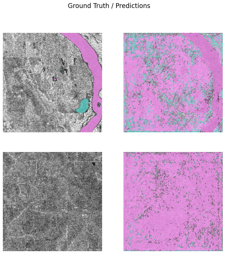
Evaluate model performance
unet.accuracy()0.17219623923301697
As we have 2 classes (1=permanent waterbodies and 2=flood water) for this segmentation task, we need to perform an accuracy assessment for each class. To achieve this, ArcGIS API for Python provides the per_class_metrics function that calculates a precision, recall, and f1 score for each class.
unet.per_class_metrics()| NoData | 1 | 2 | |
|---|---|---|---|
| precision | 0.977914 | 0.023680 | 0.006672 |
| recall | 0.169192 | 0.972512 | 0.012667 |
| f1 | 0.288475 | 0.046234 | 0.008741 |
Save the model
We will save the model that we trained as a 'Deep Learning Package' ('.dlpk' format). A Deep Learning Package is the standard format used to deploy deep learning models on the ArcGIS platform.
We will use the save() method to save the trained model. By default, it will be saved to the 'models' sub-folder within the training data folder.
unet.save('flood_model', publish=True)Computing model metrics... Published DLPK Item Id: 6b6aa1356ee64ef590f618c7d32eef92
PosixPath('/tmp/flood_inundation_mapping_using_sar_data_and_deep_learning/models/flood_model')Model inferencing
Using ArcGIS Pro, we can use the trained model on a test image/area to classify permanent waterbodies and flood inundated areas in the SAR satellite image.
After training the UnetClassifier model and saving the weights for classifying images, we can use the Classify Pixels Using Deep Learning tool tool available in ArcGIS pro and ArcGIS Enterprise for inferencing.
flood_model = gis.content.get('86d5806943024257a8a15fe17296b19b')
flood_modelraster_for_inferencing = gis.content.get('05a5c9ffd2044d2583ec1ae2a5712d54')
raster_for_inferencing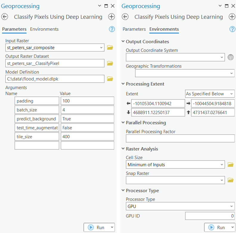
with arcpy.EnvManager(processorType="GPU"): out_classified_raster = arcpy.ia.ClassifyPixelsUsingDeepLearning("sentinel1_3band_inference_raster", "https://deldev.maps.arcgis.com/sharing/rest/content/items/86d5806943024257a8a15fe17296b19b", "padding 100;batch_size 8;predict_background True;tile_size 400", "PROCESS_AS_MOSAICKED_IMAGE", None); out_classified_raster.save(r"C:\Users\shi10484\Documents\ArcGIS\Projects\flood2\flood2.gdb\inferenced_results")
Results visualization
The classified output raster is generated using ArcGIS Pro. The output raster is published on the portal for visualization.
sar_ras2 = gis.content.get('427cd9a47eb544c59c1e965a56e72550')
inf_ras2 = gis.content.get('a7f2c8f23aa448d28fc14ec99b325ca8')
from arcgis.raster import colormap
inf_cmap2 = colormap(inf_ras2.layers[0], colormap=[[1, 7, 42, 108],[2, 0, 206, 209]])Create map widgets
Three map widgets are created showing flood inundation in different regions.
map1 = gis.map('St Peters, USA', 11)
map1.basemap='satellite'
map2 = gis.map('St Peters, USA', 11)
map2.add_layer(sar_ras2)
map3 = gis.map()
map3.add_layer(sar_ras2)
map3.add_layer(inf_cmap2)
Set the map layout
from ipywidgets import HBox, VBox, Label, Layoutmap1.sync_navigation(map2)
map2.sync_navigation(map3)Hbox and Vbox were used to set the layout of map widgets.
hbox_layout = Layout()
hbox_layout.justify_content = 'space-around'

hb1,hb2=HBox([Label('True Colour Image'),Label('Sentinel-1 Imagery'),Label('Predictions'),]),\
                HBox([Label('True Colour Image'),Label('Sentinel-1 Imagery'),Label('Predictions')])
hb1.layout,hb2.layout=hbox_layout,hbox_layout
Flood inundation mapping
The resulting predictions are provided as a map for better visualization. The results show the spatial distribution of flood water in the Midwestern US during the 2019 floods. Sentinel-1 VV imagery of May 2019 are used for the analysis. In the map widgets, it can be seen that the trained UNetClassifier model is able to identify permanent waterbodies and flood water, as well as differentiate between the two. The deep blue color represents permanent waterbodies and the cyan color represents flood water.
VBox([hb1,HBox([map1,map2,map3])])
Three map widgets were created. The left widget displays natural color high resolution satellite imagery prior to flooding, the middle widget displays the sentinel-1 imagery during the flood event, and the right map widget displays the predictions of the trained UnetClassifier model. In the maps, St Louis city can be seen where the Illinois river and the Mississippi river converge. The model is able to identify river channels and differentiate from the flood water. The True Color Imagery can be used for visual interpretation for model accuracy.
Estimation of flood inundated area (sq. km)
The pixel size of the raster is required to calculate the area of flood inundated areas. We will use the <raster>.properties.pixelSizeX and <raster>.properties.pixelSizeY functions to find the Pixel size of the raster.
## Cellsize
ras2_cellsize_x = inf_ras2.layers[0].properties.pixelSizeX
ras2_cellsize_y = inf_ras2.layers[0].properties.pixelSizeY
print(ras2_cellsize_x, ras2_cellsize_y)
14.3472971497467 14.3472971497467
To calculate the area of land under flood water, we will use the <raster>.attribute_table() function to find the count of pixels per flood water class.
inf_ras2.layers[0].attribute_table(){'fields': [{'name': 'Value',
'type': 'esriFieldTypeInteger',
'alias': 'Value',
'sqlType': 'sqlTypeOther',
'domain': None,
'defaultValue': None},
{'name': 'Count',
'type': 'esriFieldTypeDouble',
'alias': 'Count',
'sqlType': 'sqlTypeOther',
'domain': None,
'defaultValue': None},
{'name': 'Class',
'type': 'esriFieldTypeString',
'alias': 'Class',
'sqlType': 'sqlTypeOther',
'length': 1,
'domain': None,
'defaultValue': None}],
'features': [{'attributes': {'Value': 1, 'Count': 1822630, 'Class': '1'}},
{'attributes': {'Value': 2, 'Count': 5219135, 'Class': '2'}}]}This study requires the calculation of the area of land under flood water in terms of square km. The raster uses the projected coordinate system (3857), which has pixels in meters.
## area in square kilometers
area_ras2_flood_water = (5219135*(ras2_cellsize_x*ras2_cellsize_y)/1000000)
area_ras2_flood_water
1074.3325074571271
Infrastructural inundation assessment
The inferenced raster will be used to assess the infrasruture inundated in flood water.
flood_raster = Raster("https://tiledimageservices6.arcgis.com/SMX5BErCXLM7eDtY/arcgis/rest/services/st_louis_flood_water/ImageServer",
                      gis=gis_ent,
                      engine="image_server")
The LULC raster for St. Louis is generated using the Land Cover Classification (Sentinel-2) pretrained model to assess the inundated areas per the LULC class.
lulc_raster = Raster("https://tiledimageservices6.arcgis.com/SMX5BErCXLM7eDtY/arcgis/rest/services/lulc_st_louis/ImageServer",
                        gis=gis_ent,
                        engine="image_server")
The flood raster will be converted to polygons using convert_raster_to_feature. We then use the import_data function to create a new feature layer containing the flood water polygons.
flood_poly = convert_raster_to_feature(flood_raster,
                                    field='Value',
                                    output_type='Polygon',
                                    simplify=False,
                                    output_name='flood_st_louis_poly'+str(datetime.datetime.now().microsecond),
                                    gis=gis)

## Create dataframe from feature layer and get water polygons
dfm1 = flood_poly.layers[0].query('gridcode=2').sdf

## Convert dataframe to feature layer
flood_poly = gis.content.import_data(dfm1, title='flood_water_poly'+str(datetime.datetime.now().microsecond))
Next, the LULC raster will be converted to polygons using convert_raster_to_feature. After getting the LULC polygons, we remove NODATA and Water polygons and use the import_data function to create a new feature layer containing the correct LULC polygons.
lulc_poly = convert_raster_to_feature(lulc_raster,
                                    field='Value',
                                    output_type='Polygon',
                                    simplify=False,
                                    output_name='lulc_st_louis_poly'+str(datetime.datetime.now().microsecond),
                                    gis=gis)

## Create dataframe from feature layer and get water polygons
dfm2 = lulc_poly.layers[0].query('gridcode > 0 And gridcode < 5').sdf

## Convert dataframe to feature layer
lulc_polygon = gis.content.import_data(dfm2, title='lulc_poly'+str(datetime.datetime.now().microsecond))
To get the LULC classes for the flood inundated areas, we will use the overlay_layers function.
inundated_lulc = overlay_layers(lulc_polygon.layers[0],
                                flood_poly.layers[0],
                                output_name='inundated_lulc'+str(datetime.datetime.now().microsecond),
                                gis=gis)
{"cost": 72.43}
After getting the LULC classes for the flood inundated areas, we will dissolve the polygons on the basis of gridcode. The output feature layer will have the combined area of each class in square miles units.
lulc_dissolve = dissolve_boundaries(inundated_lulc,
                               dissolve_fields=['gridcode'],
                               output_name='dissolved_lulc'+str(datetime.datetime.now().microsecond),
                               gis=gis,
                               multi_part_features=True)
{"cost": 9.685}
The resulting feature layer has a column for the area per class, but the corresponding LULC class name is missing. We will add the class names to the dataframe using the code below.
dfm4 = lulc_dissolve.layers[0].query().sdf
lulc_classes = ['Artificial surfaces', 'Agricultural areas', 'Forest and semi natural areas', 'Wetlands']
dfm4['LULC_Classes'] = lulc_classes
dfm5 = dfm4[['gridcode','AnalysisArea', 'LULC_Classes']].copy()
dfm5.rename(columns={'AnalysisArea': 'Area_in_square_miles'}, inplace=True)
dfm5| gridcode | Area_in_square_miles | LULC_Classes | |
|---|---|---|---|
| 0 | 1 | 7.469743 | Artificial surfaces |
| 1 | 2 | 189.190674 | Agricultural areas |
| 2 | 3 | 5.561292 | Forest and semi natural areas |
| 3 | 4 | 14.224226 | Wetlands |
Conclusion
In this notebook, we have demonstrated how to use a UnetClassifier model with ArcGIS API for Python to extract flood water and permanent waterbodies. In Part 1, we covered how Sentinel-1 SAR data can be used for flood inundation mapping and monitoring. This process involved steps to prepare the input data, train a pixel-based classification model, visualize the results, generate accuracy metrics, and inferencing results on a test raster/area. Finally, in Part 2, we demonstrated the flood water inundated area in square kilometers and an infrastructural inundation assessment.
