- 🔬 Data Science
- 🥠 Deep Learning and image translation
Introduction
Land Surface Temperature (LST) plays an important role in the Earth’s climate system. It represents the process of energy exchange, affecting both water content and vegetation growth rate. Traditionally, LST from Landsat-8 is calculated using a chain of formulas that are complex and demanding of resources. Fortunately, deep learning models provide an efficient way to compute and predict LST. In this study, we propose an approach to predicting LST from Landsat 8 imagery using the Pix2Pix deep learning model. The LST will be computed on a thermal band (band 10) from a single Landsat 8 image. The calculated LST will then be used to train an image translation Pix2Pix model. The model will then be capable of translating Landsat-8 multispectral imagery to LST, allowing the predictions to be used for multitemporal monitoring of LST.
Necessary imports
import os
from pathlib import Path

from arcgis import GIS
from arcgis.learn import Pix2Pix, prepare_data
Connect to your GIS
gis = GIS('home')Export image domain data
A stacked raster of Landsat-8 bands has been created using bands 1-7 and band 10. This mosaic will be used as our input_raster for the training data.
landsat_mosaic = gis.content.get('952468e0942c4b6893006cb267cbf040')
landsat_mosaicThe raster for Land Surface Temperature is generated using the thermal band (band 10). This raster will be used as the Additional Input Raster for the training data.
lst_raster = gis.content.get('ad29f8ab93354e77bcb22ba83f9a846a')
lst_rasterMethodology
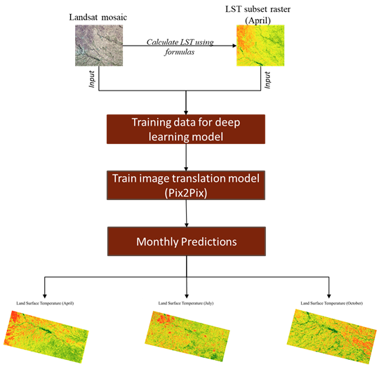
The diagram above encapsulates the overall methodology used in the estimation of the Land Surface Temperature from multispectral imagery using deep learning.
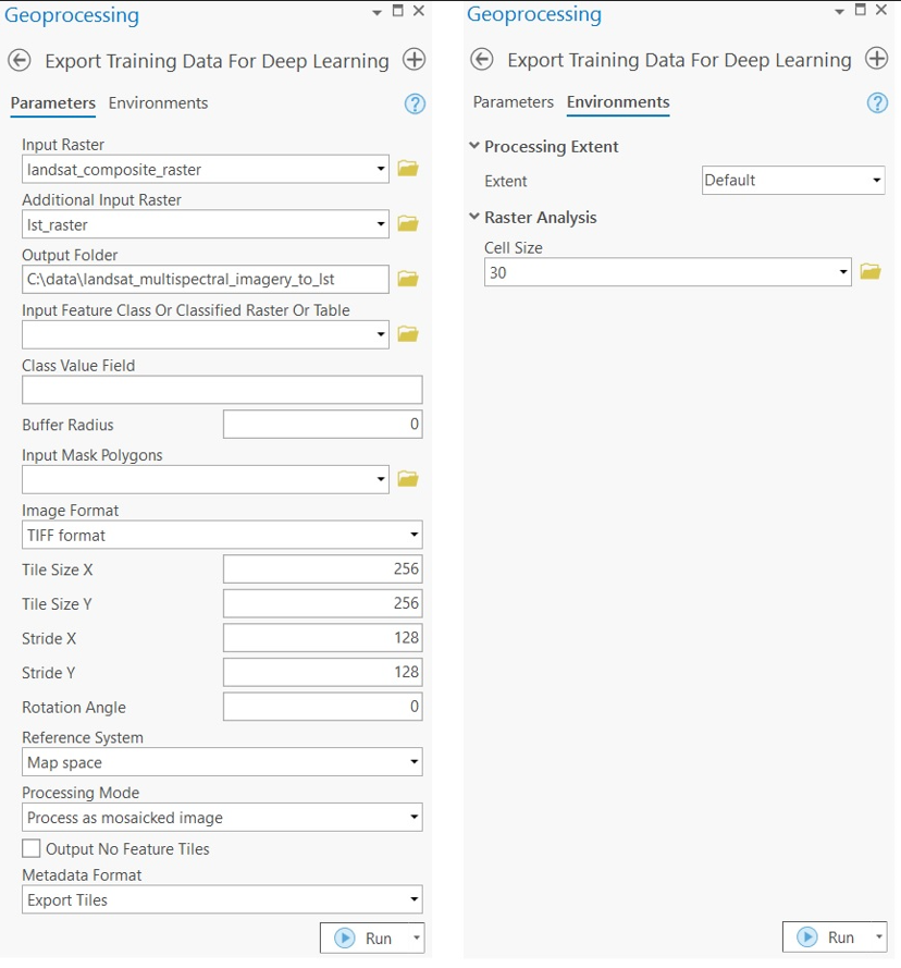
The data will be exported in the “Export_Tiles” metadata format, which is available in the Export Training Data For Deep Learning tool. This tool is available in ArcGIS Pro and ArcGIS Image Server. The various inputs required by the tool are described below:
-
Input Raster: landsat_composite_raster -
Additional Input Raster: lst_raster -
Tile Size X & Tile Size Y: 256 -
Stride X & Stride Y: 128 -
Meta Data Format: 'Export_Tiles' (as we are training aPix2Pixmodel). -
Environments: Set optimumCell Size,Processing Extent.
Inside the exported data folder, the 'Images' and 'Images2' folders contain all of the image tiles from the two domains exported from landsat_composite_raster and lst_raster respectively.
Model training
Alternatively, we have provided a subset of training data containing a few samples that follow the same directory structure mentioned above and that provides the rasters used for exporting the training dataset. This data can be used to run the experiments.
training_data = gis.content.get('11ebeb485c2d44898b32b91b105f8de6')
training_datafilepath = training_data.download(file_name=training_data.name)#Extract the data from the zipped image collection
import zipfile
with zipfile.ZipFile(filepath, 'r') as zip_ref:
zip_ref.extractall(Path(filepath).parent)Prepare data
output_path = Path(os.path.join(os.path.splitext(filepath)[0]))data = prepare_data(output_path, dataset_type="Pix2Pix", batch_size=8)Visualize a few samples from your training data
To get a sense of what the training data looks like, the arcgis.learn.show_batch() method randomly picks a few training chips and visualizes them. Below, the images displayed on the left are Landsat-8 rasters, and the images on the right are the corresponding LST rasters.
data.show_batch()
Load model architecture
model = Pix2Pix(data)Tuning for optimal learning rate
Learning rate is one of the most important hyperparameters in model training. ArcGIS API for Python provides a learning rate finder that automatically chooses the optimal learning rate for you.
lr = model.lr_find()
lr
6.309573444801929e-05
Fit the model
Next, the model is trained for 30 epochs with the suggested learning rate.
model.fit(30, lr)| epoch | train_loss | valid_loss | gen_loss | l1_loss | D_loss | time |
|---|---|---|---|---|---|---|
| 0 | 35.566357 | 30.796040 | 0.663380 | 0.349030 | 0.717529 | 01:05 |
| 1 | 19.291725 | 12.093425 | 0.622104 | 0.186696 | 0.742149 | 01:08 |
| 2 | 11.148993 | 8.225349 | 0.592061 | 0.105569 | 0.758912 | 01:11 |
| 3 | 7.698595 | 6.032180 | 0.579509 | 0.071191 | 0.764611 | 01:13 |
| 4 | 5.424048 | 3.987901 | 0.581081 | 0.048430 | 0.762080 | 01:12 |
| 5 | 3.604111 | 3.223908 | 0.593590 | 0.030105 | 0.753615 | 01:13 |
| 6 | 2.858333 | 2.664019 | 0.600027 | 0.022583 | 0.749187 | 01:14 |
| 7 | 2.528771 | 2.296279 | 0.604608 | 0.019242 | 0.746166 | 01:13 |
| 8 | 2.322142 | 2.211593 | 0.607804 | 0.017143 | 0.743662 | 01:13 |
| 9 | 2.194105 | 2.021927 | 0.608942 | 0.015852 | 0.742633 | 01:13 |
| 10 | 2.062931 | 1.906173 | 0.614715 | 0.014482 | 0.738948 | 01:16 |
| 11 | 1.974658 | 1.963890 | 0.617611 | 0.013570 | 0.736867 | 01:13 |
| 12 | 1.884406 | 1.913554 | 0.617948 | 0.012665 | 0.735938 | 01:14 |
| 13 | 1.812625 | 1.689833 | 0.621684 | 0.011909 | 0.733461 | 01:15 |
| 14 | 1.761084 | 1.651570 | 0.623631 | 0.011375 | 0.731869 | 01:14 |
| 15 | 1.785958 | 1.609133 | 0.622693 | 0.011633 | 0.732524 | 01:14 |
| 16 | 1.686648 | 1.601160 | 0.625848 | 0.010608 | 0.730283 | 01:15 |
| 17 | 1.651397 | 1.583226 | 0.626592 | 0.010248 | 0.729233 | 01:09 |
| 18 | 1.561778 | 1.554424 | 0.629964 | 0.009318 | 0.726959 | 01:09 |
| 19 | 1.537263 | 1.492239 | 0.631422 | 0.009058 | 0.726120 | 01:09 |
| 20 | 1.549876 | 1.467906 | 0.633227 | 0.009166 | 0.725323 | 01:12 |
| 21 | 1.473448 | 1.468675 | 0.634735 | 0.008387 | 0.724095 | 01:10 |
| 22 | 1.458049 | 1.544640 | 0.636126 | 0.008219 | 0.723233 | 01:10 |
| 23 | 1.408463 | 1.401212 | 0.638078 | 0.007704 | 0.722065 | 01:10 |
| 24 | 1.385678 | 1.389169 | 0.638943 | 0.007467 | 0.721458 | 01:09 |
| 25 | 1.381514 | 1.419574 | 0.639691 | 0.007418 | 0.721018 | 01:10 |
| 26 | 1.375896 | 1.382134 | 0.640013 | 0.007359 | 0.720693 | 01:10 |
| 27 | 1.357910 | 1.366140 | 0.640478 | 0.007174 | 0.720604 | 01:10 |
| 28 | 1.348851 | 1.366569 | 0.640338 | 0.007085 | 0.720462 | 01:12 |
| 29 | 1.343235 | 1.369570 | 0.640250 | 0.007030 | 0.720480 | 01:10 |
Here, with 30 epochs, we can see reasonable results, as both the training and validation losses have gone down considerably, indicating that the model is learning to translate between imagery domains.
Save the model
Next, we will save the trained model as a 'Deep Learning Package' ('.dlpk' format). The Deep Learning package format is the standard format used to deploy deep learning models on the ArcGIS platform.
We will use the save() method to save the trained model. By default, it will be saved to the 'models' sub-folder within our training data folder.
model.save("pix2pix_model", publish=True, overwrite=True)Published DLPK Item Id: a94c729d87774b5e92a25d344e25364f
WindowsPath('C:/Users/shi10484/AppData/Local/Temp/models/pix2pix_model')Visualize results in validation set
It is a good practice to see the results of the model viz-a-viz the ground truth. The code below selects random samples and displays the ground truth and model predictions side by side. This enables us to preview the results of the model within the notebook.
model.show_results(rows=4)
Compute evaluation metrics
To objectively assess the synthesized image quality obtained from the model generators, we will quantitatively evaluate the results using the Structural Similarity (SSIM) Index and the Peak Signal-to-Noise Ratio (PSNR).
The SSIM index measures the structural information similarity between images, with 0 indicating no similarity and 1 indicating complete similarity. The SSIM value for the trained model is 0.94.
The PSNR measures image distortion and noise level between images. A 20 dB or higher PSNR indicates that the image is of good quality. The PSNR value for the trained model is 20.9.
model.compute_metrics(){'PSNR': '2.0965e+01', 'SSIM': '9.4536e-01'}Model inferencing
After training the Pix2Pix model and saving the weights for translating images, we can use the Classify Pixels Using Deep Learning tool, available in both ArcGIS pro and ArcGIS Enterprise, for inferencing at scale.
model_for_inferencing = gis.content.get('a94c729d87774b5e92a25d344e25364f')
model_for_inferencing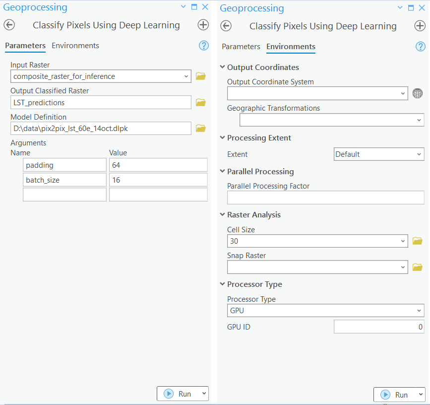
with arcpy.EnvManager(processorType="GPU"): out_classified_raster = arcpy.ia.ClassifyPixelsUsingDeepLearning("composite_raster_for_inferencing", r"C:\path\to\model.dlpk", "padding 64;batch_size 8;predict_background True; tile_size 224", "PROCESS_AS_MOSAICKED_IMAGE", None); out_classified_raster.save(r"C:\sample\sample.gdb\predicted_lst")
Results visualization
Here, the LST for the months of April and July are generated using ArcGIS Pro. The output rasters are then published on our portal for visualization.
inferenced_results_april = gis.content.get('b52f79a31c994dc0ac30aec41733e564')
inferenced_results_aprilfrom arcgis.raster.functions import colormap, stretch
inf_apr_lyr = inferenced_results_april.layers[0]
stretch_rs_apr = colormap(stretch(inf_apr_lyr,
stretch_type='PercentClip',
min=0,
max=255),
colormap_name="Condition Number")inferenced_results_july = gis.content.get('d02bc8947de64aee9a448a215a70bc94')
inferenced_results_julyinf_july_lyr = inferenced_results_july.layers[0]
stretch_rs_july = colormap(stretch(inf_july_lyr,
stretch_type='PercentClip',
min=0,
max=255),
colormap_name="Condition Number")Create map widgets
Next, two map widgets are created showing the Landsat 8 mosaic and Inferenced LST raster.
map1 = gis.map('Iowa, USA')
map1.zoom = 13
map1.content.add(stretch_rs_apr)
map2 = gis.map('Iowa, USA')
map2.zoom = 13
map2.content.add(stretch_rs_july)
map3 = gis.map('Iowa, USA')
map3.zoom = 13
map3.basemap.basemap = 'satellite'
map1.zoom_to_layer(stretch_rs_apr)
Synchronize web maps
Once created, the maps can be synchronized with each other using the MapView.sync_navigation functionality. By syncing the two map widgets, we can more easily compare the inferenced results with the DSM. A more detailed description of advanced map widget options can be found here.
map1.sync_navigation(map2)
map2.sync_navigation(map3)map1.zoom_to_layer(stretch_rs_apr)Set the map layout
from ipywidgets import HBox, VBox, Label, LayoutHbox and Vbox were used to set the layout of map widgets.
hbox_layout = Layout()
hbox_layout.justify_content = 'space-around'

hb1,hb2,hb3=HBox([Label('April')]),\
            HBox([Label('July')]),\
            HBox([Label('RGB Imagery')])
hb1.layout,hb2.layout,hb3.layout=hbox_layout,hbox_layout,hbox_layout
Results
The predictions are provided as a map for better visualization.
VBox([hb1,HBox([map1]),hb2,HBox([map2]), hb3,HBox([map3])])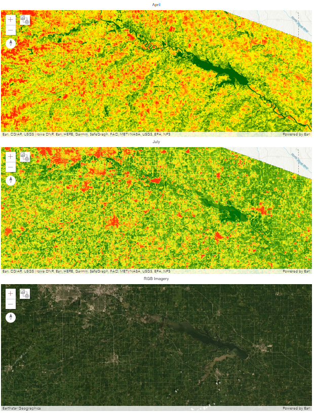
map2.zoom_to_layer(stretch_rs_apr)In the maps above, the land surface temperature increases from dark green to red. The corn crop is usually sown in late April or early May, therefore, in the month of April, there will be little to no crop. This can be seen in April's prediction, where most of the area is yellow or orange in color, indicating a high land surface temperature. However, in the month of July, the crop is fully grown, resulting in the predictions for most of the area being dark or light green in color.
Conclusion
In this notebook, we have demonstrated how to use a Pix2Pix model using ArcGIS API for Python to translate imagery from one domain to another.


