Landsat 8 to Sentinel-2 using Pix2Pix

Introduction

The Landsat program is the longest running mission for the acquisition of satellite imagery of the earth. The images acquired have opened multiple doors for studies observing the earth. In 2015, Sentinel-2, with 10 m resolution imagery, further enhanced our ability to study and observe the earth. Now, with the advancements in deep learning techniques, there is a need to revisit historic images from the Landsat program and increase their resolution to perform studies at a higher resolution.

In this sample notebook, we will see how we can make use of the Pix2Pix model to convert 30 meter resolution Landsat 8 imagery to 10 meter resolution Sentinel-2 imagery, thus allowing us to use Landsat 8 imagery for processes like precision agriculture.

Necessary imports

import os, zipfile
from pathlib import Path

from arcgis.gis import GIS
from arcgis.learn import prepare_data, Pix2Pix

gis = GIS(profile = "your_online_profile")

Export training data

For this example, we will be using both Landsat 8 and Sentinel-2 imagery. We have exported this data in a “Export_Tiles” metadata format, available in the Export Training Data For Deep Learning tool. This Export Training Data For Deep Learning tool is available in ArcGIS Pro and ArcGIS Image Server.

Input Raster: Landsat 8 imagery
Additional Raster: Sentinel-2 imagery
Tile Size X & Tile Size Y: 256
Stride X & Stride Y: 128
Meta Data Format: 'Export_Tiles', as we are training a Pix2Pix model.
Environments: Set Cell Size as 10 to convert Landsat 8 imagery to Sentinel-2 imagery with a 10m resolution.

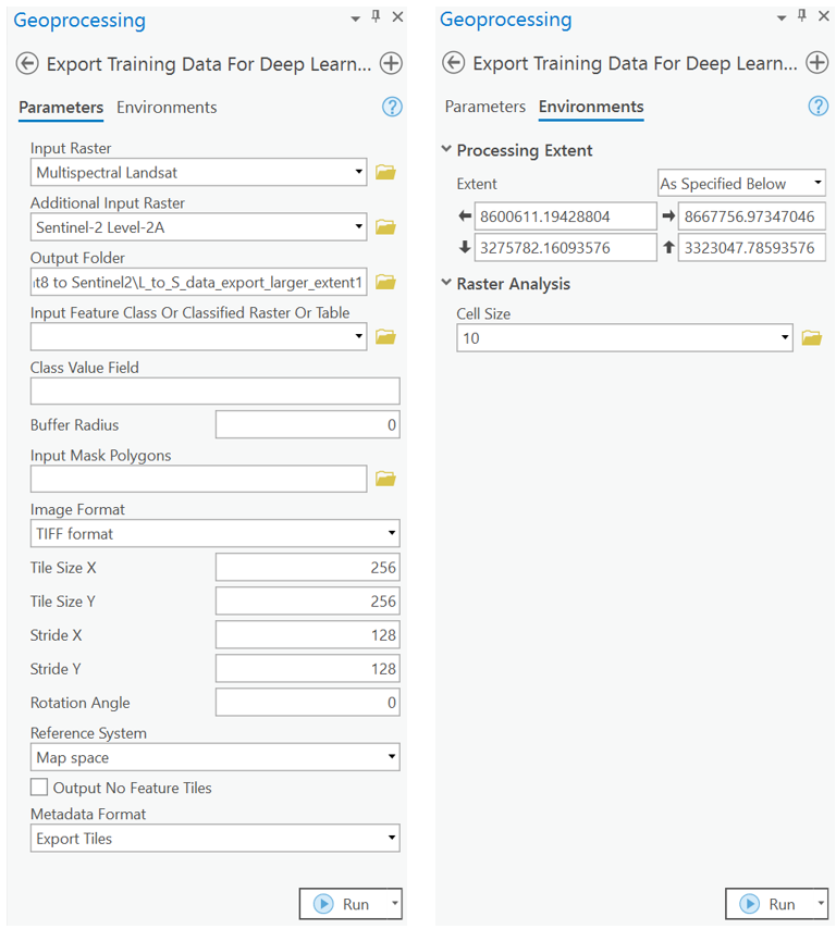
Here is the link to the sample data exported by following the steps mentioned above.

output_l1 = r"./Landsat8 to Sentinel2"
if not os.path.exists(output_l1):
    os.mkdir(output_l1)

output_l2 = r"./Landsat8 to Sentinel2/L_to_S_data_export_larger_extent"
if not os.path.exists(output_l2):
    os.mkdir(output_l2)

sample_data = gis.content.get("40b1bae898c441c9832d9dd15a73ab70")
sample_data.download(save_path=output_l2)

'/arcgis/home/Landsat8 to Sentinel2/L_to_S_data_export_larger_extent/Exported_Data_Landsat_to_Sentinel_10.zip'

zf = zipfile.ZipFile(os.path.join(output_l2, 'Exported_Data_Landsat_to_Sentinel_10.zip'))
zf.extractall(path = os.path.join(output_l2, ''))

Train the model

Prepare the data

Here, we will specify the path to our training data and a few hyperparameters.

path: path of the folder containing the training data.
batch_size: The number of images your model will train on each step inside an epoch. This directly depends on the memory of your graphic card. 64 worked for us on a 32GB GPU.

output_path = r"./Landsat8 to Sentinel2/L_to_S_data_export_larger_extent/Exported_Data_Landsat_to_Sentinel_10"
data = prepare_data(output_path, batch_size=64)

Visualize the training data

To get a sense of what the training data looks like, the arcgis.learn.show_batch() method will randomly select a few training chips and visualize them.

rows: The number of rows to visualize

data.show_batch(rows=2)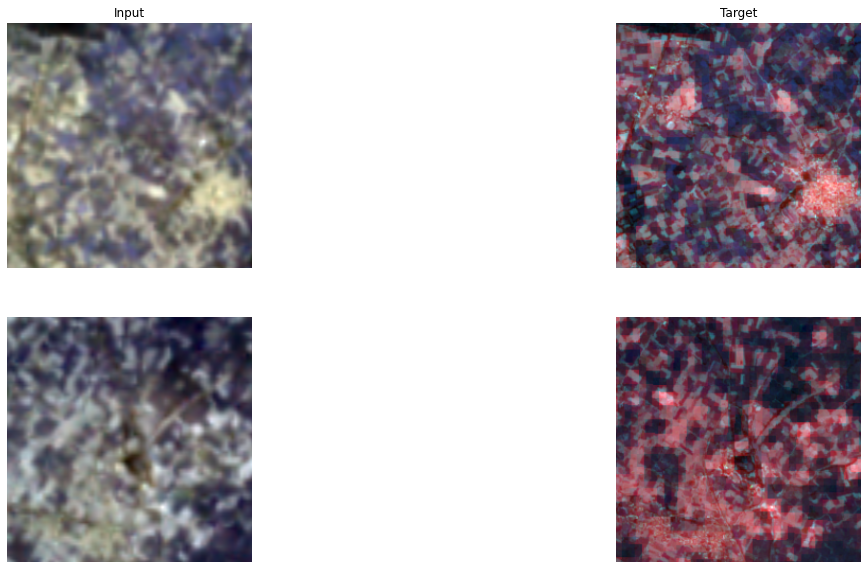

Load the model architecture

model = Pix2Pix(data)

Find an optimal learning rate

Learning rate is one of the most important hyperparameters in model training. The ArcGIS API for Python provides a learning rate finder that will automatically select the optimal learning rate for you.

lr = model.lr_find()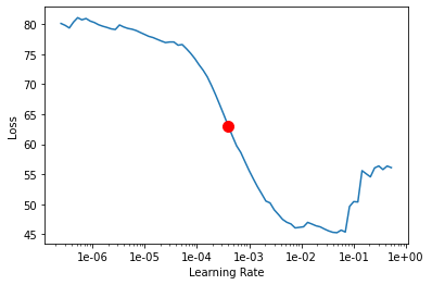

Fit the model

Next, we will train the model for a few epochs with the learning rate found above.

model.fit(100, lr=lr)

epoch	train_loss	valid_loss	gen_loss	l1_loss	D_loss	time
0	67.922554	101.058823	0.806639	0.671159	0.888794	04:38
1	52.827030	78.936195	0.788984	0.520380	0.882063	04:25
2	38.657383	63.050945	0.780396	0.378770	0.877670	04:24
3	28.062674	58.513496	0.779523	0.272831	0.874605	04:24
4	21.155628	56.853664	0.774855	0.203808	0.870376	04:35
5	16.308531	56.166840	0.765249	0.155433	0.866498	04:37
6	14.429462	55.781639	0.753477	0.136760	0.863398	04:40
7	12.368107	55.496456	0.740846	0.116273	0.860481	04:42
8	11.972437	55.270863	0.727483	0.112450	0.858373	04:42
9	11.420366	55.159748	0.715936	0.107044	0.856639	04:43
10	10.366476	55.061447	0.705256	0.096612	0.855376	04:44
11	10.210399	55.001419	0.696726	0.095137	0.853653	04:29
12	9.475751	54.880295	0.694076	0.087817	0.851885	04:41
13	9.763708	54.692776	0.689342	0.090744	0.850283	04:43
14	9.226028	54.739616	0.686319	0.085397	0.848299	04:39
15	9.124137	54.590904	0.681929	0.084422	0.845997	04:41
16	9.700657	54.605179	0.678598	0.090221	0.843811	04:44
17	9.803352	54.466850	0.674727	0.091286	0.841702	04:38
18	9.250247	54.443752	0.671712	0.085785	0.838615	04:39
19	8.335964	54.438122	0.668105	0.076679	0.836434	04:41
20	7.968552	54.415028	0.663330	0.073052	0.833919	04:39
21	7.480053	54.328480	0.660825	0.068192	0.830940	04:39
22	6.977783	54.422703	0.658739	0.063190	0.827839	04:38
23	8.002518	54.275131	0.656007	0.073465	0.825168	04:23
24	8.120469	54.323711	0.653857	0.074666	0.821486	04:36
25	8.971378	54.200165	0.653120	0.083183	0.818777	04:37
26	8.524234	54.223305	0.650678	0.078736	0.815513	04:39
27	7.693572	54.175900	0.650067	0.070435	0.811447	04:38
28	7.585774	54.169350	0.648958	0.069368	0.808204	04:42
29	7.294562	54.193363	0.648175	0.066464	0.804726	04:39
30	7.423637	54.142086	0.647378	0.067763	0.801125	04:41
31	7.691103	54.132977	0.646267	0.070448	0.798250	04:40
32	8.032001	54.186432	0.645121	0.073869	0.795223	04:40
33	7.716933	54.023232	0.645245	0.070717	0.792041	04:37
34	7.807978	54.097683	0.646286	0.071617	0.788926	04:38
35	7.054918	54.051414	0.645621	0.064093	0.785243	04:40
36	7.364428	54.043598	0.646439	0.067180	0.782689	04:41
37	7.992309	54.106018	0.646157	0.073462	0.780123	04:42
38	7.756326	54.019592	0.646435	0.071099	0.778077	04:39
39	7.377257	54.013203	0.646747	0.067305	0.775721	05:04
40	7.501619	53.944485	0.647765	0.068539	0.773242	04:41
41	7.908170	53.996967	0.647310	0.072609	0.771274	04:38
42	7.076623	53.970837	0.648404	0.064282	0.768852	04:41
43	6.944644	53.927929	0.649475	0.062952	0.766984	04:40
44	6.451814	54.015945	0.651909	0.057999	0.764742	04:39
45	6.648439	54.031849	0.653823	0.059946	0.762842	04:35
46	6.862483	53.894760	0.655473	0.062070	0.761267	04:26
47	6.540757	53.850662	0.657263	0.058835	0.759471	04:38
48	6.772334	53.889977	0.658314	0.061140	0.757680	04:36
49	6.989652	53.831516	0.660464	0.063292	0.755698	04:37
50	7.044950	53.878418	0.662366	0.063826	0.754088	04:39
51	6.799073	53.820854	0.662351	0.061367	0.752575	04:41
52	6.428719	53.830032	0.663130	0.057656	0.751407	04:40
53	6.398839	53.770561	0.663466	0.057354	0.750302	04:39
54	6.196313	53.789524	0.665439	0.055309	0.748688	04:39
55	7.442753	53.382652	0.665368	0.067774	0.747504	04:37
56	7.595248	53.354031	0.665322	0.069299	0.746258	04:39
57	6.784313	53.242893	0.665820	0.061185	0.744622	04:38
58	6.327766	53.229862	0.667371	0.056604	0.743340	04:39
59	7.045929	53.223110	0.669550	0.063764	0.741719	04:44
60	6.687289	53.209389	0.669957	0.060173	0.740586	04:40
61	6.500633	53.232124	0.671055	0.058296	0.739568	04:40
62	6.583332	53.285110	0.671405	0.059119	0.738427	04:41
63	6.972293	53.251854	0.671564	0.063007	0.737322	04:41
64	6.807597	53.192921	0.672022	0.061356	0.735825	04:39
65	6.949701	53.234032	0.671913	0.062778	0.734925	04:42
66	6.992170	53.353321	0.671870	0.063203	0.734017	04:40
67	6.417209	53.187592	0.671373	0.057458	0.733351	04:39
68	6.815023	53.160919	0.670866	0.061442	0.732577	04:46
69	7.495409	53.132549	0.672304	0.068231	0.731766	04:32
70	6.964630	53.139645	0.672781	0.062919	0.730722	04:33
71	7.159966	53.126362	0.674060	0.064859	0.730159	04:34
72	7.181245	53.168339	0.675254	0.065060	0.729455	04:37
73	6.733634	53.172653	0.675814	0.060578	0.728774	04:36
74	7.289911	53.151363	0.676047	0.066139	0.728120	04:37
75	7.498312	53.091747	0.676542	0.068218	0.727649	04:37
76	7.427543	53.079216	0.676691	0.067509	0.727156	04:38
77	6.536768	53.106808	0.677548	0.058592	0.726407	04:38
78	6.337427	53.073940	0.678534	0.056589	0.725822	04:40
79	6.977967	53.095291	0.678463	0.062995	0.725427	04:40
80	7.065238	53.060497	0.678638	0.063866	0.724829	04:42
81	7.163990	53.070633	0.679182	0.064848	0.724701	04:43
82	7.803146	53.093517	0.679920	0.071232	0.724518	04:47
83	6.781487	53.054237	0.679795	0.061017	0.723992	04:52
84	6.674012	53.054031	0.680461	0.059936	0.723873	04:49
85	5.713095	53.054295	0.680950	0.050321	0.723741	04:53
86	5.723894	53.048443	0.681045	0.050428	0.723395	04:41
87	5.978154	53.027294	0.681104	0.052970	0.723122	04:35
88	5.876119	53.032894	0.681088	0.051950	0.722766	04:38
89	6.553662	53.038715	0.681061	0.058726	0.722940	04:35
90	7.407327	53.024139	0.681787	0.067255	0.723052	04:39
91	7.021692	53.020111	0.682331	0.063394	0.722830	04:38
92	6.479682	53.017532	0.682917	0.057968	0.722677	04:37
93	5.853846	53.017826	0.682270	0.051716	0.722154	04:27
94	6.393230	53.015102	0.682149	0.057111	0.722446	04:34
95	7.152648	53.018314	0.682215	0.064704	0.722553	04:39
96	6.646112	53.019951	0.682040	0.059641	0.722465	04:35
97	6.610269	53.019367	0.682215	0.059281	0.722389	04:37
98	6.449659	53.017513	0.682448	0.057672	0.722295	04:36
99	6.107530	53.017139	0.682420	0.054251	0.722165	04:35

Here, with 100 epochs, we can see reasonable results, as both the training and validation losses have gone down considerably. This indicates that the model is learning to translate Landsat 8 imagery to Sentinel-2.

Visualize the results in validation set

It is a good practice to see results of the model viz-a-viz the ground truth. The code below picks random samples and displays the ground truth and model predictions side by side. This enables us to preview the results of the model within the notebook.

model.show_results(2)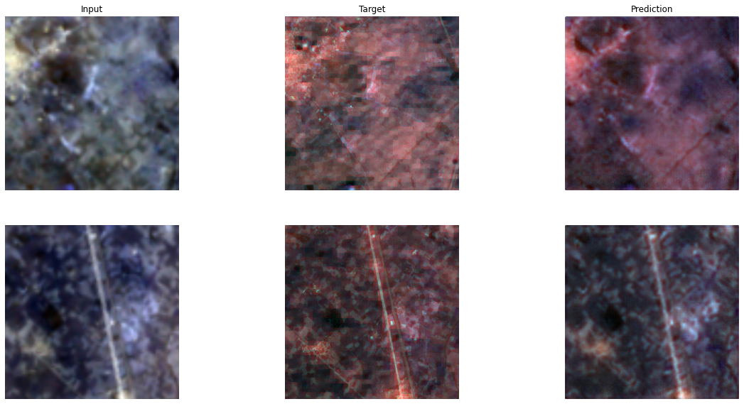

Generative Adversarial Network (GAN) models require a significant amount time to train, and even with the initial 100 epochs trained so far, there is still room for more training. As such, we trained this model for an additional 400 epochs (500 in total), to achieve good results. With the additional training, the training and validation losses dropped to 5.45 and 52.6 respectively and the D_loss stabilized at 0.54.

Below is the loss curve, which represents the training and validation losses during the training process.

model.plot_losses()

Save the model

Next, we will save the trained model as a 'Deep Learning Package' ('.dlpk' format). Deep Learning package is the standard format used to deploy deep learning models on the ArcGIS platform.

We will use the save() method to save the trained model. By default, it will be saved to the 'models' sub-folder within our training data folder.

model.save("Landsat_to_Sentinel_LE_500e")

Computing model metrics...

WindowsPath('D:/Landsat8 to Sentinel2/L_to_S_data_export_larger_extent/models/Landsat_to_Sentinel_LE_500e')

Model inference

In this step, we will generate a classified raster using the 'Classify Pixels Using Deep Learning' tool available in both ArcGIS Pro and ArcGIS Enterprise.

Input Raster: The raster layer you want to classify.
Model Definition: Located inside the saved model in the 'models' folder in '.emd' format.
Padding: The 'Input Raster' is tiled, and the deep learning model classifies each individual tile separately before producing the final 'Output Classified Raster'. This may lead to unwanted artifacts along the edges of each tile, as the model has little context to predict accurately. Padding allows us to supply extra information along the tile edges, thus helping the model to make better predictions.
Cell Size: Should be close to the size used to train the model.
Processor Type: Allows you to control whether the system's 'GPU' or 'CPU' will be used to classify pixels. By default, 'GPU' will be used if available.

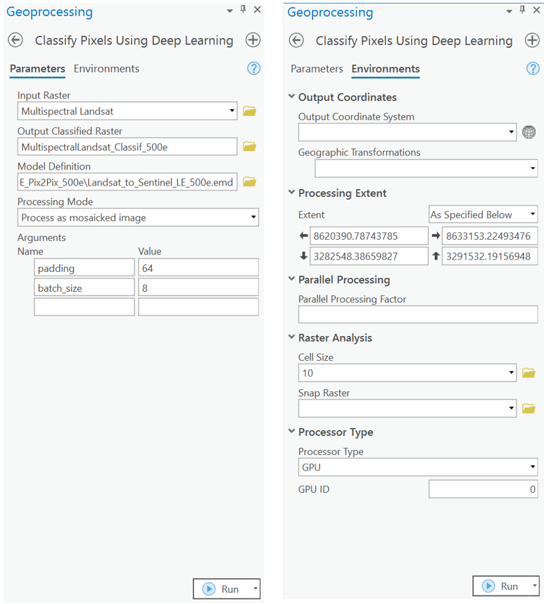
It is advised to zoom in to the right extent of the area of interest in order to avoid/reduce noise from the results as the model is not trained to be generalized to work across the globe.

Results

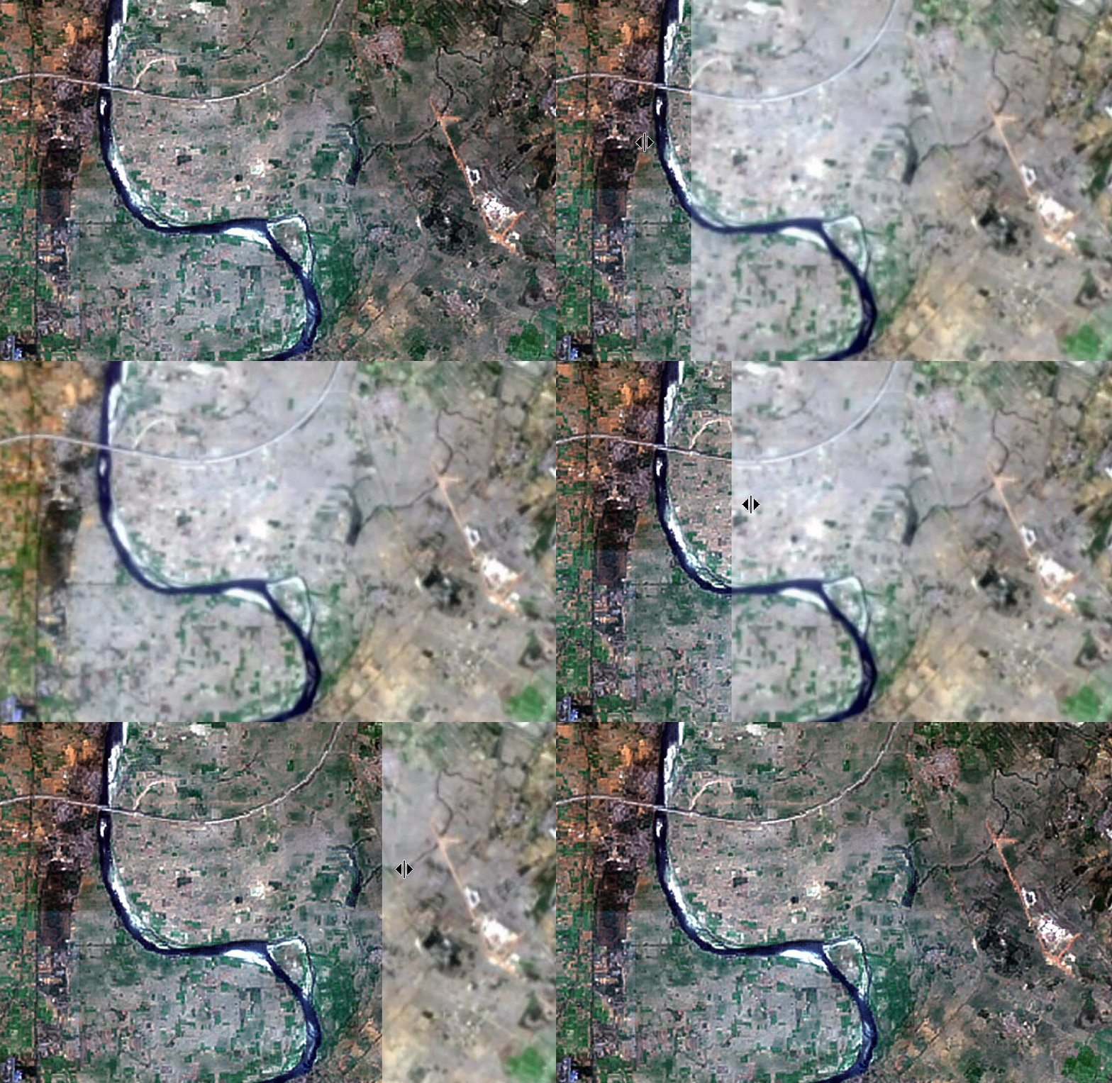
The gif below was achieved with the model trained in this notebook. The model converted a Landsat 8 image with a 30m resolution to an image with a 10m resolution and 15 bands, similar to Sentinel-2 images.

Below is the same generated image viewed through the agriculture band combination of SWIR-1 (B11), near-infrared (B8), and blue (B2). This band combination can be used to monitor the health of crops.

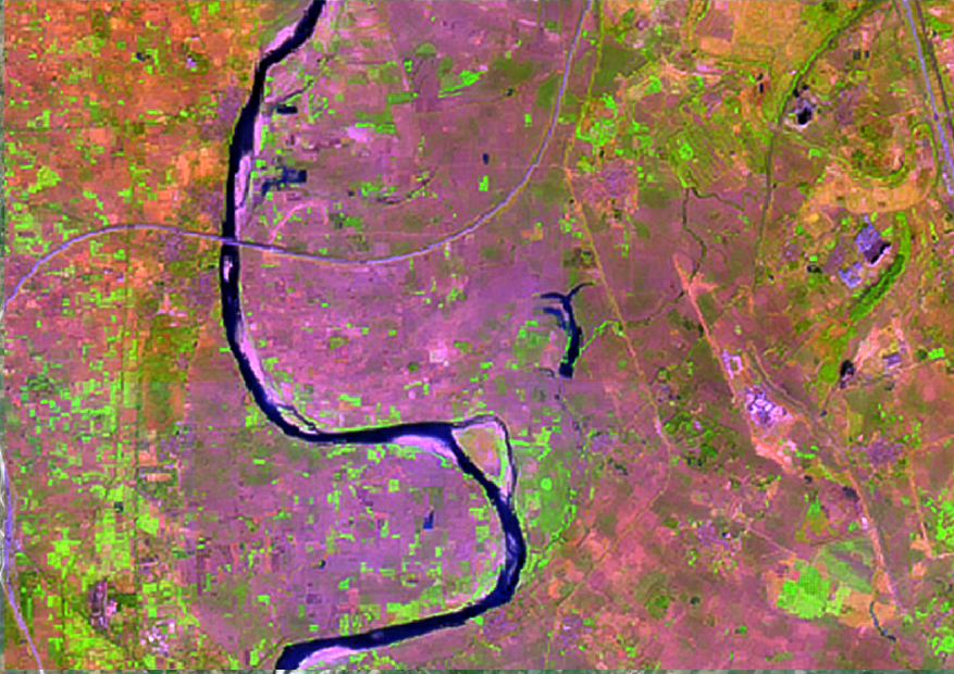
Here, the dark green patches highlight dense vegetation and healthy crops.

Conclusion

In this notebook, we have demonstrated how to use the Pix2Pix model, available in the ArcGIS API for Python, to translate Landsat 8 imagery to Sentinel-2 imagery.

References

[1] How Pix2Pix works ?, https://developers.arcgis.com/python/guide/how-pix2pix-works/.